Predicting health information avoidance using machine learning models

Introduction

Health information avoidance—defined as any behavior designed to prevent or delay access to available but potentially unwanted health information (Howell, Lipsey, and Shepperd (2020); Sweeny et al. (2010))—remains a significant barrier to realizing the public health benefits of personalized risk communication. Despite the rapid expansion of access to medical information in the Information Age, many people still choose not to learn about their personal health risks (Gigerenzer and Garcia-Retamero (2017); Ho, Hagmann, and Loewenstein (2021); Kelly and Sharot (2021)). Health information avoidance is not a uniform behavior, but can take multiple forms, varying in its duration and degree of intentionality. Individuals may avoid health information by delaying the decision to learn about their screening results or they may avoid it completely, choosing to never know. Information avoidance may also manifest through both active and passive means. People may explicitly ask others not to disclose information, physically remove themselves from situations were information might be revealed, or passively refrain from questions that could reveal unwanted knowledge. These avoidance behaviors may manifest as refusing cancer screening, delaying medical care, or not requesting test results (Sweeny et al. (2010)).

Research indicates that health information avoidance is common. For example, approximately 15% of US adults avoid personalized health risk information across various contexts (Meese et al., 2022), and nearly 39% express a reluctance to learn about their cancer risk (Emanuel et al. (2015)). Similar avoidance rates (e.g., approximately 40%) have been observed for non-personalized health information (i.e., general health information not relevant to personal risk) (Chae, Lee, and Kim (2019); Orom et al. (2020)).

Such widespread avoidance underscores the need to understand how and why individuals avoid health information. Some individuals may avoid health information to protect themselves from unpleasant emotions, prevent exposure to information that conflicts with their worldview or creates an obligation to act. Even when the information may be critical to health,avoidance eliminates the discomfort of decision-making and the emotional burden of confronting potential illness (Sweeny et al. (2010)). Previous research has identified various psychological and cognitive factors underlying this avoidance phenomenon and explored potential explanations for this behavior. O’Brien et al. (2024) found that self-perceptions of health, such as low perceived risk, engagement in healthy behaviors, and demographic characteristics, often guide people’s decisions to avoid learning about their health risks. Other studies have shown that information overload can increase anxiety and cognitive dissonance, leading to avoidance behavior (Dattilo et al. (2022); Song, Yao, and Wen (2021); Soroya and Faiola (2023)). Furthermore, heightened risk perceptions can exacerbate anxiety and sadness, which may further hinder people from seeking health information (Sultana, Dhillon, and Oliveira (2023); Zhao and Cai (2009)).

However, few studies have attempted to use machine learning methods to identify predictors of health information avoidance. This study applies predictive modeling and machine learning methods to examine patterns of cancer screening avoidance (“health avoiders”) using sociodemographic and psychological data. By integrating behavioral and belief factors, this study aimed to better understand the complex dynamics that lead to health information avoidance.

Review of Machine Learning Methods

Machine learning (ML) methods were applied to identify patterns associated with health information avoidance. Each model differs in complexity, interpretability, and suitability for different types of data structures. This study focuses on three main models: Logistic Regression, Random Forest, and Multivariate Adaptive Regression Splines (MARS). Each approach offers different advantages and trade-offs, summarized in Table 1 below.

Table 1. Comparison of Machine Learning Models

Model	Description	Advantages	Limitations	Interpretability
Linear Regression	Models the relationship between predictors and a continuous outcome using a straight-line equation.	Simple, interpretable, and efficient to train; effective for linearly related data; allows understanding of variable relationships.	Assumes linearity and independence among variables; sensitive to outliers; limited for complex or nonlinear data.	High
Logistic Regression	Estimates the probability of a binary outcome based on a linear combination of predictors.	Simple, interpretable, good baseline; easy to assess predictor importance.	Assumes linearity; struggles with nonlinear or high-dimensional data.	High
Random Forest	Ensemble of decision trees using bootstrapped samples and random feature selection.	Handles nonlinear and complex data; reduces overfitting; provides feature importance.	Less interpretable; slower with large datasets; harder to explain model logic.	Moderate
MARS (Multivariate Adaptive Regression Splines)	Builds flexible regression models using piecewise linear splines.	Captures nonlinear relationships; performs automatic feature selection; minimal preprocessing needed.	Computationally intensive; interpretation can be challenging with correlated predictors.	Moderate - High

In summary, Linear / Logistic Regression provides transparency and simplicity, Random Forest offers high predictive power for complex data, and MARS strikes a balance between flexibility and interpretability.

So in our study, Linear / Logistic Regression served as a baseline interpretable model, Random Forest captured complex nonlinear interactions, and MARS modeled adaptive spline-based relationships between predictors and cancer avoidance. By comparing these models, this study aimed to identify the most effective approach to predict health information avoidance while maintaining interpretability.

Method

Data Source

This study used the de-identified Health Avoiders dataset provided through Cloud Research in collaboration with Dr. Heather Orom (University at Buffalo). The dataset includes sociodemographic, psychological, and behavioral variables collected under IRB approval managed by Dr. Shane McCarty. All analyses were conducted in R, and reproducibility was ensured through a version-controlled Git repository and Quarto documentation workflow.

Outcome Variable

The outcome variable, Cancer_Avoidance_Mean, represents the average score across 8 items (Avoid_Cancer_)measuring participants’ avoidance of cancer-related health information. Because this variable exhibited non-normality, both logarithmic and square-root transformations were tested; however, these transformations did not improve model performance or interpretability, so the untransformed variable was retained for analysis.

Predictor Models

Heather Orom (University at Buffalo) developed a theoretical framework to group predictors as a health psychologist studying health information avoidance.

1. Demographic Model — Ethnicity, Political_Party, Gender4, Job_Classification, Education_Level, Age, Income, Race, and MacArthur_Numeric.

2. Media Use Model — Social_Media_Usage, AI_Use, Video_Games_Hours, Listening_Podcasts, Facebook_Usage_num, TikTok_Use, X_Twitter_Usage, Social_Media_type, and Influencer_Following.

3. Health Condition Model — Stressful_Events_Recent, Current_Depression, Anxiety_Severity_num, PTSD5_Score, Health_Depression_Severity_num, and Stress_TotalScore.

4. Health Behavior Model — Fast_Food_Consumption, Meditation_group, Physical_Activity_Guidelines, Cigarette_Smoking_num, Supplement_Consumption_Reason_num, Diet_Type, and Supplement_Consumption.

5. Other Factors Model — Home_Ownership, Voter_Registration, Climate_Change_Belief, and Mental_Health_of_Partner.

Variable Scaling and Scoring

Several psychological and health condition variables were standardized using validated scales:

• PC-PTSD-5: a 5-item yes/no screen for post-traumatic stress.

• GAD-7: a 7-item measure of anxiety severity (0–3 scale).

• PHQ-9: a 9-item measure of depression severity (0–3 scale).

• Life Events Checklist: summed to represent cumulative stress exposure.

Composite averages were computed for each domain, resulting in 4 continuous variables: PTSD5_Score, Anxiety_Severity_num, Health_Depression_Severity_num, and Stress_TotalScore.

Analysis Plan

Predictive modeling was conducted in R using the tidymodels package. Due to the non-normal outcome variable, two complimentary approaches were applied:

1. Regression Models: predicted the continuous outcome Cancer_Avoidance_Mean were fitted using Linear Regression (baseline), Random Forest, and Multivariate Adaptive Regression Splines (MARS). Model performance was assessed using root mean squared error (RMSE), mean absolute error (MAE), and the correlation between predicted and observed values.

2. Classification Models: predicted the binary outcome Cancer_Avoiders01 (0 = non-avoider, 1 = avoider) were fitted using Logistic Regression (baseline) and Random Forest. Model performance was assessed using area under the curve (AUC) and accuracy with basic calibration applied when class imbalance occurred.

Some models used cross-validation, and Linear / Logistic Regression served as the baseline for comparison.

Results

All analyses were conducted in Posit Cloud, a collaborative online platform for writing R scripts and developing Quarto markdown documents.

IMPORT

In [1]:

library(tidymodels)

── Attaching packages ────────────────────────────────────── tidymodels 1.1.0 ──

✔ broom        1.0.5     ✔ recipes      1.3.1
✔ dials        1.2.0     ✔ rsample      1.1.1
✔ dplyr        1.1.2     ✔ tibble       3.2.1
✔ ggplot2      3.4.2     ✔ tidyr        1.3.0
✔ infer        1.0.4     ✔ tune         1.1.1
✔ modeldata    1.2.0     ✔ workflows    1.1.3
✔ parsnip      1.1.0     ✔ workflowsets 1.0.1
✔ purrr        1.0.2     ✔ yardstick    1.2.0

── Conflicts ───────────────────────────────────────── tidymodels_conflicts() ──
✖ purrr::discard() masks scales::discard()
✖ dplyr::filter()  masks stats::filter()
✖ dplyr::lag()     masks stats::lag()
✖ recipes::step()  masks stats::step()
• Dig deeper into tidy modeling with R at https://www.tmwr.org

library(ranger)

In [2]:

library(readr)

Attaching package: 'readr'

The following object is masked from 'package:yardstick':

    spec

The following object is masked from 'package:scales':

    col_factor

alldata <-
  read_csv("data/alldata.csv") %>%
  mutate(across(where(is.character), as.factor))

Rows: 11219 Columns: 108

── Column specification ────────────────────────────────────────────────────────
Delimiter: ","
chr (107): US Veteran, Ethnicity, Monolingual, Migrant Status, Household Com...
dbl   (1): Age

ℹ Use `spec()` to retrieve the full column specification for this data.
ℹ Specify the column types or set `show_col_types = FALSE` to quiet this message.

TRANSFORM

Predictors

In [3]:

selectdata <- alldata %>%
  select("Ethnicity", "Political Party", "Gender", "Job Classification", "Education", 
         "Age", "Personal Income", "Race", "MacArthur Scale", "Social Media Usage", "AI Use", 
         'Video Games Hours', "Listening to Podcasts", "Facebook Usage", "Frequency of TikTok Use", 
         "X (Twitter) Usage", "Social Media", "Influencer Following",
         "Stressful Events - Reaction", "Stressful Events - Guilt", "Stressful Events - Detachment",
         "Stressful Events - Nightmares", "Stressful Events - Avoiding Situations",
         "Stressful Events - Recent Occurence", "Current Depression", 
         "Anxiety - Trouble Relaxing", "Anxiety - Irritable", "Anxiety - Restlessness",
         "Anxiety - Feeling Afraid", "Anxiety - Nervousness", "Anxiety - Worrying", 
         "Health - Feeling Failure", "Health - Hopelessness", "Health - Feeling Tired",
         "Health - Interest In Things", "Health - Pace", "Health - Poor Appetite",
         "Health - Thoughts Of Self Infliction", "Health - Concentration", "Health - Trouble Sleeping",
         "Anxiety - Worrying Different Things", "Stress Related Events - Most Stressful", "Stress Related Events",
         "Medical Diagnoses In Life", "Fast Food Consumption", "Physical Activity Guidelines", "Cigarette Smoking",
         "Supplement Consumption Reason", "Vaccinations", "Diet Type", "Supplement Consumption", "Meditation", 
         "Home Ownership", "Voter Registration", "Climate Change Belief", "Mental Health of Partner",
         "Information Avoidance - Cancer 1", "Information Avoidance - Cancer 2", 
         "Information Avoidance - Cancer 3 (R)", "Information Avoidance - Cancer 4", 
         "Information Avoidance - Cancer 5 (R)", "Information Avoidance - Cancer 6", 
         "Information Avoidance - Cancer 7 (R)", "Information Avoidance - Cancer 8 (R)") %>%
  rename(
    Political_Party = `Political Party`,
    Job_Classification = `Job Classification`,
    Personal_Income = `Personal Income`,
    MacArthur_Scale = `MacArthur Scale`,
    
    Social_Media_Usage = `Social Media Usage`,
    AI_Use = `AI Use`,
    Video_Games_Hours = `Video Games Hours`,
    Listening_Podcasts = `Listening to Podcasts`,
    Facebook_Usage = `Facebook Usage`,
    TikTok_Use = `Frequency of TikTok Use`,
    X_Twitter_Usage = `X (Twitter) Usage`,
    Social_Media_type =  `Social Media`,
    Influencer_Following = `Influencer Following`,
    
    Stressful_Events_Reaction = `Stressful Events - Reaction`,
    Stressful_Events_Guilt = `Stressful Events - Guilt`,
    Stressful_Events_Detachment = `Stressful Events - Detachment`,
    Stressful_Events_Nightmares = `Stressful Events - Nightmares`,
    Stressful_Events_Avoiding_Situations = `Stressful Events - Avoiding Situations`,
    Stressful_Events_Recent = `Stressful Events - Recent Occurence`,
    Current_Depression = `Current Depression`,
    Stressful_Events_Detachment = `Stressful Events - Detachment`,
    
    Anxiety_Trouble_Relaxing = `Anxiety - Trouble Relaxing`,
    Anxiety_Irritable = `Anxiety - Irritable`,
    Anxiety_Restlessness = `Anxiety - Restlessness`,
    Anxiety_Feeling_Afraid = `Anxiety - Feeling Afraid`,
    Anxiety_Nervousness = `Anxiety - Nervousness`,
    Anxiety_Worrying = `Anxiety - Worrying`,
    
    Health_Feeling_Failure = `Health - Feeling Failure`,
    Health_Hopelessness = `Health - Hopelessness`,
    Health_Feeling_Tired = `Health - Feeling Tired`,
    Health_Interest_In_Things = `Health - Interest In Things`,
    Health_Pace = `Health - Pace`,
    Health_Poor_Appetite = `Health - Poor Appetite`,
    Health_Thoughts_Of_Self_Infliction = `Health - Thoughts Of Self Infliction`,
    Health_Concentration = `Health - Concentration`,
    Health_Trouble_Sleeping = `Health - Trouble Sleeping`,
    Anxiety_Worrying_Different_Things = `Anxiety - Worrying Different Things`,
    
    Stressful_Events_Most = `Stress Related Events - Most Stressful`,
    Stress_Related_Events = `Stress Related Events`,
    Medical_Diagnoses_In_Life = `Medical Diagnoses In Life`,
    
    Fast_Food_Consumption = `Fast Food Consumption`,
    Physical_Activity_Guidelines = `Physical Activity Guidelines`,
    Cigarette_Smoking = `Cigarette Smoking`,
    Supplement_Consumption_Reason = `Supplement Consumption Reason`,
    Diet_Type = `Diet Type`,
    Supplement_Consumption = `Supplement Consumption`,
    
    Home_Ownership = `Home Ownership`,
    Voter_Registration = `Voter Registration`,
    Climate_Change_Belief = `Climate Change Belief`,
    Mental_Health_of_Partner = `Mental Health of Partner`
  )

In [4]:

selectdata <- selectdata %>%
  mutate(
    across(where(is.character), as.factor),
    Ethnicity = factor(Ethnicity, levels = c(
      "Yes, Cuban",
      "No, not of Hispanic, Latino, or Spanish origin",
      "Yes, Mexican, Mexican Am., Chicano",
      "Yes, another Hispanic, Latino, or Spanish origin – (for example, Salvadoran, Dominican, Colombian, Guatemalan, Spaniard, Ecuadorian, etc.)",
      "Yes, Puerto Rican",
      "Prefer not to say")),
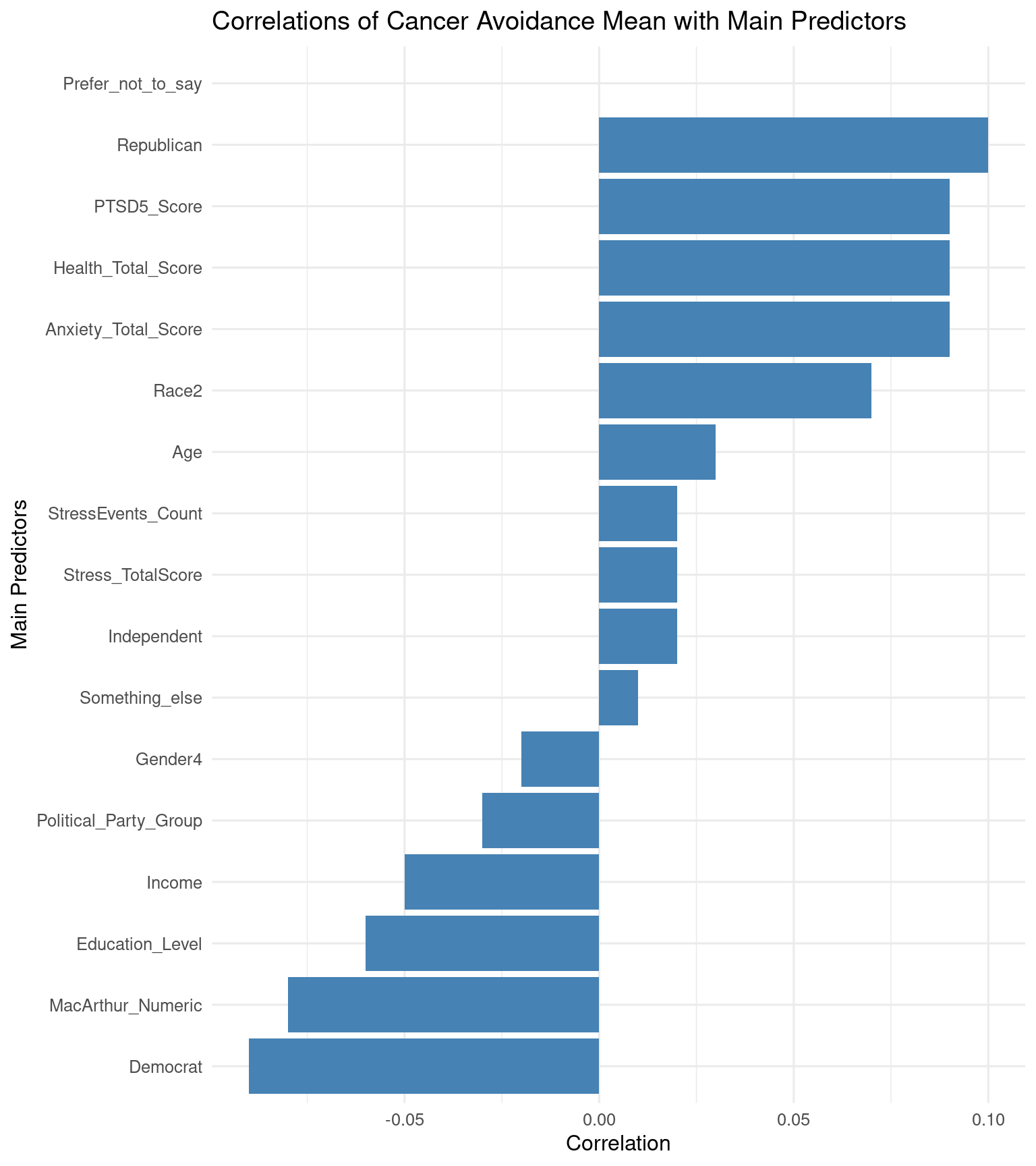
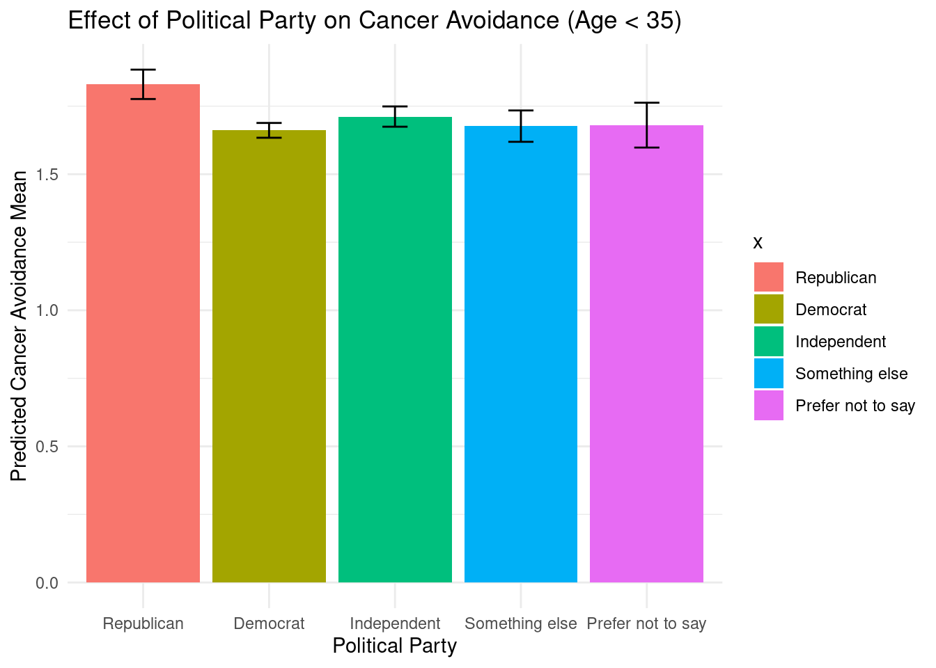
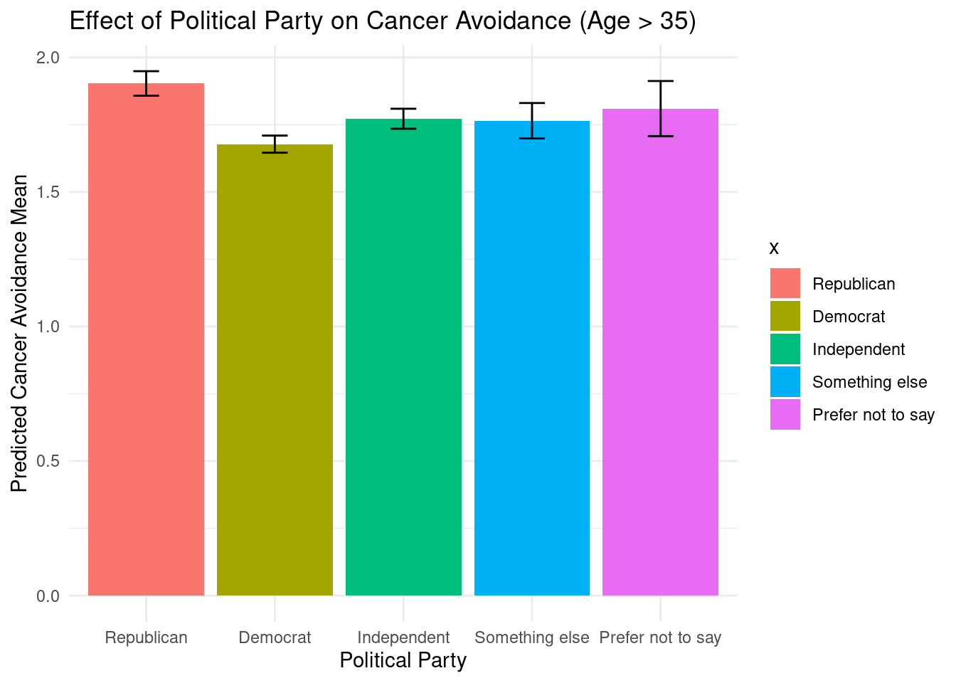
    Political_Party = factor(Political_Party, levels = c(
      "Republican", "Democrat", "Independent", "Something else", "Prefer not to say")),
    Gender = factor(Gender, level = c(
        "Woman",
        "Man",
        "Non-binary",
        "Agender",
        "Two-spirit",
        "Additional gender category/identity not listed",
        "Prefer not to say")),
    Job_Classification = factor(Job_Classification, levels = c(
      "White Collar (e.g., accountant, software developer, human resources manager, marketing analyst, public safety)", "Creative or Cultural (e.g., writer, artist, musician, actor)", "Public Service and Government (e.g., soldier, teacher, police officer, public health worker, education, childcare)", "Information Technology (e.g., IT specialist, web developer, data scientist, cybersecurity analyst)", "Service Industry (e.g., retail worker, server, hotel staff, flight attendant, food services, personal care, funeral services, animal/veterinary care, leisure and hospitality)", "Freelance and Gig Economy (e.g., freelance writer, graphic designer, rideshare driver, delivery person)", "Blue Collar (e.g., electrician, plumber, mechanic, welder, manufacturing, oil and gas extraction, transportation, utilities, mining, waste collection/treatment/disposal, automotive services)", "Professional (e.g., doctor, lawyer, professor, engineer, nurse, healthcare)", "I am unemployed/a student/stay at home parent", " Manual Labor (e.g., farmer, construction worker, factory worker, miner, landscaping, agriculture, cleaning and custodial services)")),
    Education = factor(Education, levels = c(
      "No formal education",
      "Less than a high school diploma",
      "High school graduate - high school diploma or the equivalent (for example: GED)",
      "Some college, but no degree",
      "Associate degree (for example: AA, AS)",
      "Bachelor's degree (for example: BA, AB, BS)",
      "Master's degree (for example: MA, MS, MEng, MEd, MSW, MBA)",
      "Professional degree (for example: MD, DDS, DVM, LLB, JD)",
      "Doctorate degree (for example: PhD, EdD)",
      "Prefer not to say")),
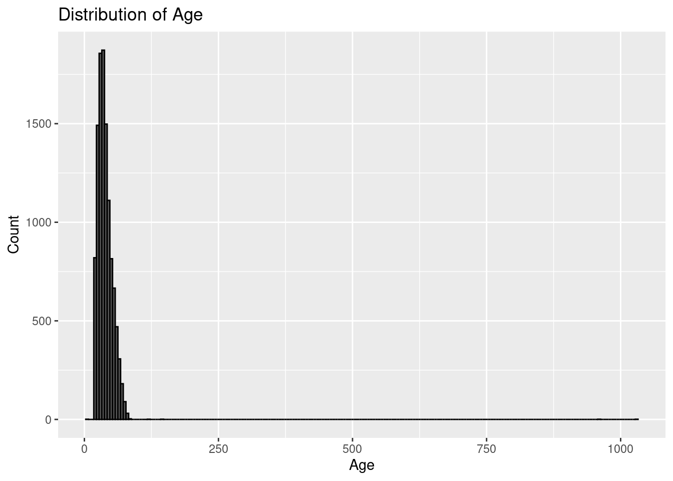
     AgeGroup = case_when(
      Age < 25 ~ "18–24",
      Age < 35 ~ "25–34",
      Age < 45 ~ "35–44",
      Age < 55 ~ "45–54",
      Age < 65 ~ "55–64",
      TRUE     ~ "65+"
    ),
    AgeGroup = factor(AgeGroup, levels = c("18–24", "25–34", "35–44", "45–54", "55–64", "65+")),
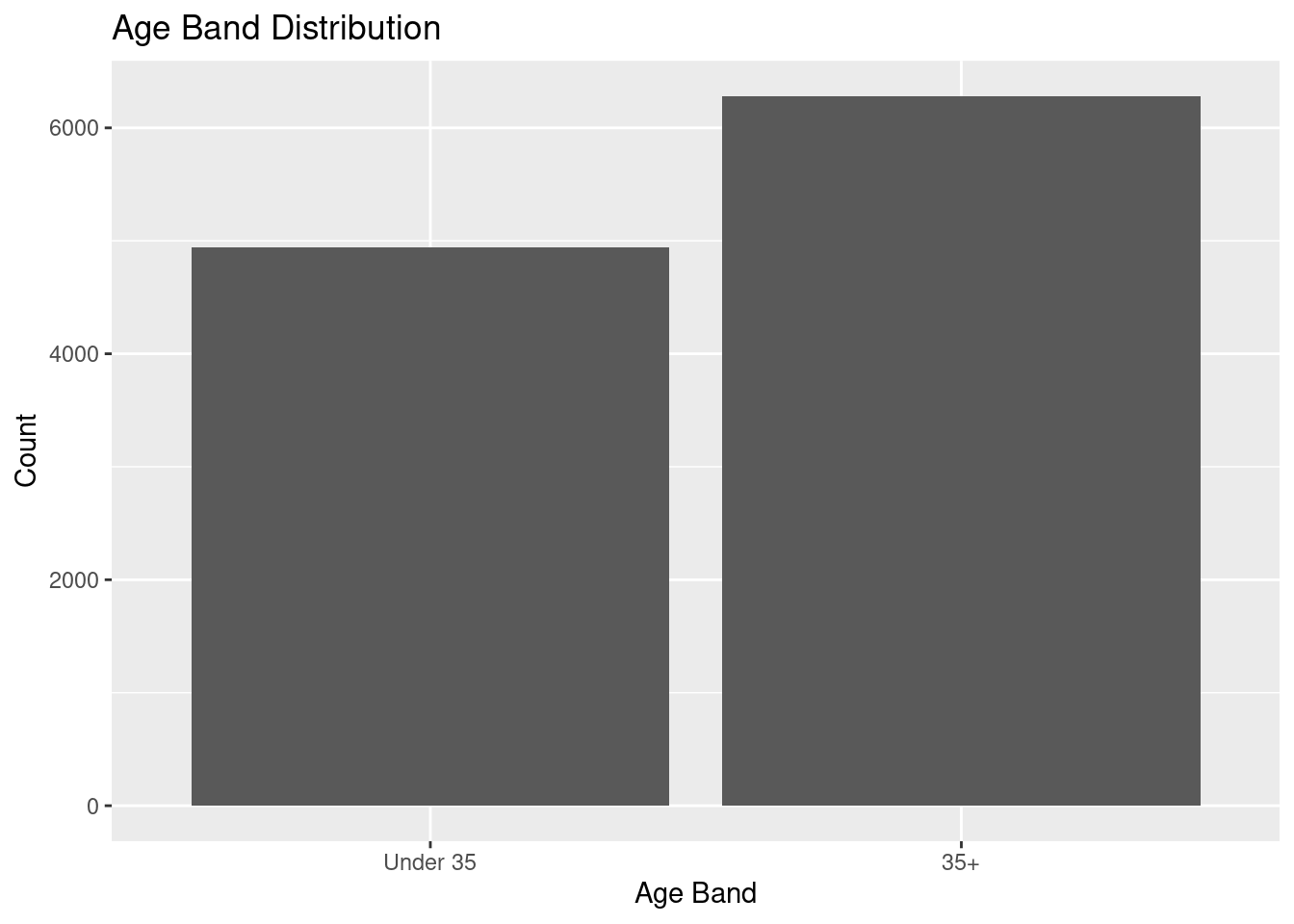
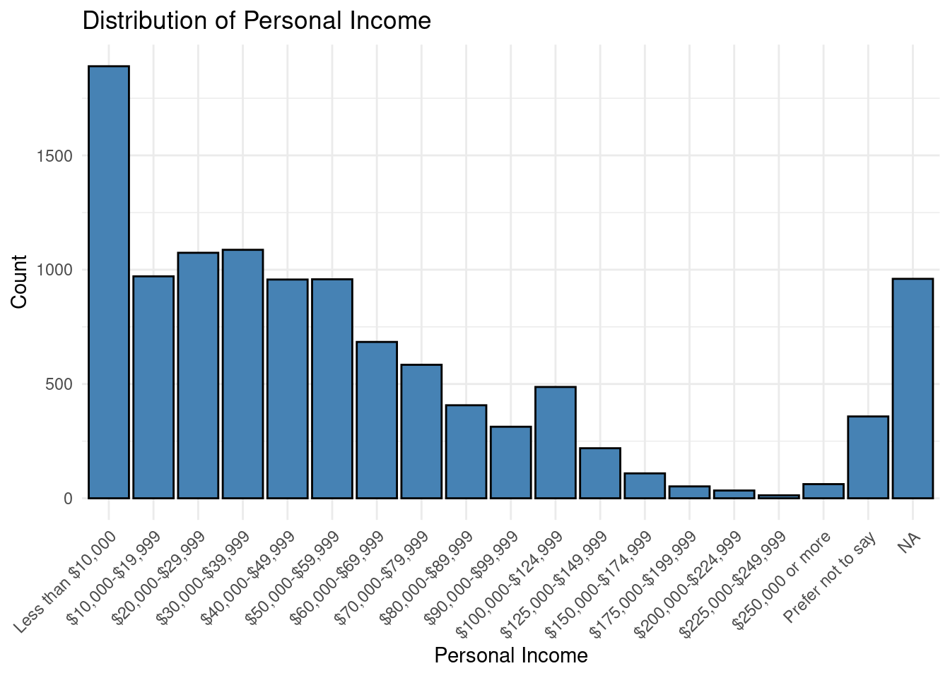
    Personal_Income = factor(Personal_Income, levels = c(
      "Less than $10,000",
        "$10,000-$19,999",
        "$20,000-$29,999",
        "$30,000-$39,999",
        "$40,000-$49,999",
        "$50,000-$59,999",
        "$60,000-$69,999",
        "$70,000-$79,999",
        "$80,000-$89,999",
        "$90,000-$99,999",
        "$100,000-$124,999",
        "$125,000-$149,999",
        "$150,000-$174,999",
        "$175,000-$199,999",
        "$200,000-$224,999",
        "$225,000-$249,999",
        "$250,000 or more",
        "Prefer not to say")),
    Race = factor(Race, levels = c(
    "American Indian or Alaska Native",
    "Asian Indian", "Chinese", "Filipino", "Japanese", "Korean", "Vietnamese", "Samoan", "Guamanian", "Hawaiian",
    "Black or African American",
    "White",
    "An ethnicity not listed here",
    "Other",
    "Prefer not to say")),
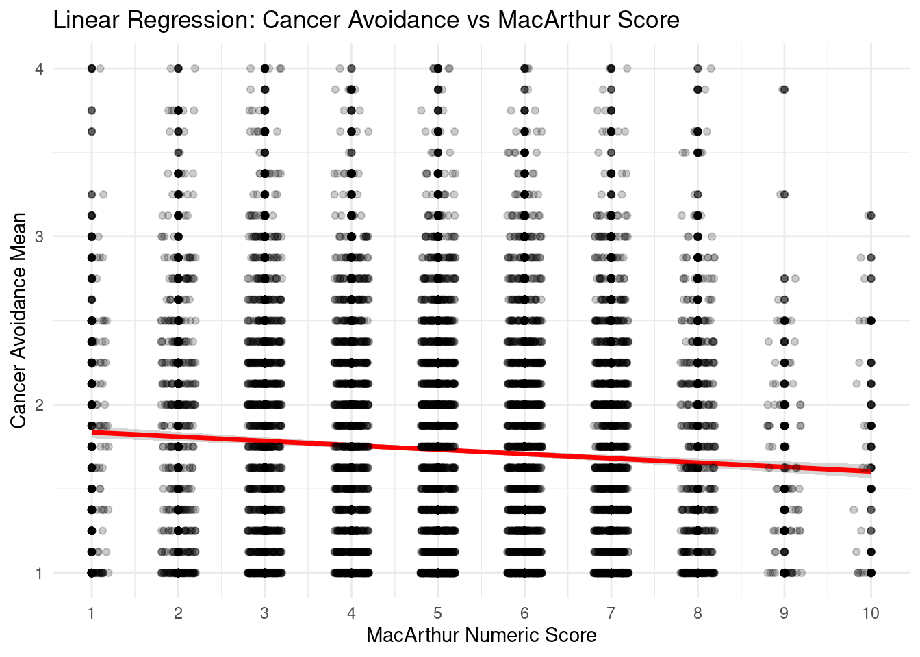
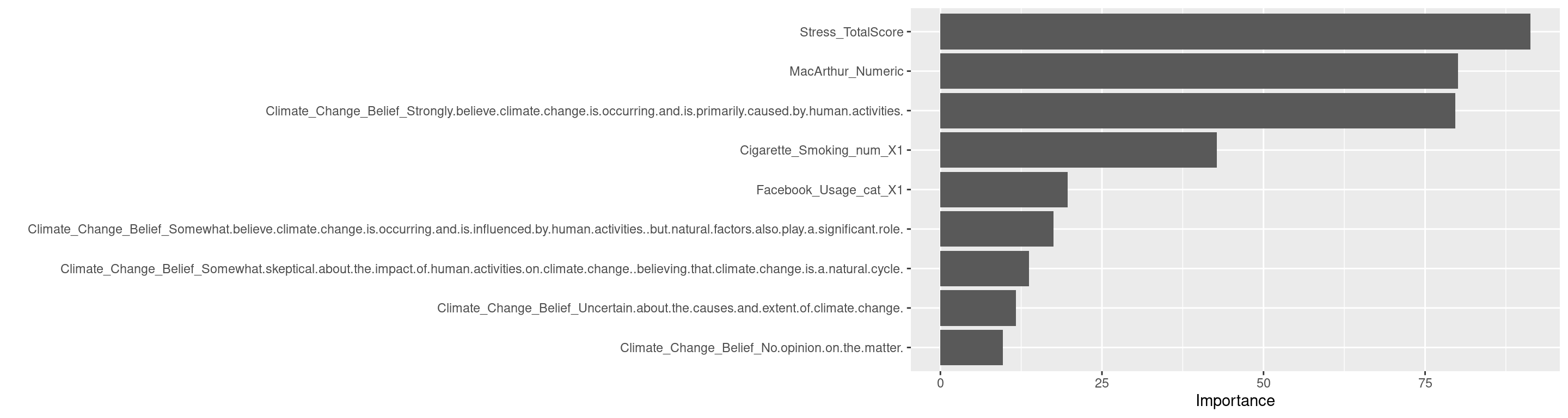
    MacArthur_Scale = factor(MacArthur_Scale, levels = paste("Rung", 1:10)),
    Social_Media_Usage = factor(Social_Media_Usage, levels = c(
             "Never",
             "A couple of times a year",
             "A couple of times a month",
             "Every week",
             "Every day")),
    Listening_Podcasts = factor(Listening_Podcasts, levels = c(
    "I have never listened to a podcast",
    "I do not regularly listen to podcasts",
    "At least every 4 weeks (22-30 days)",
    "At least every 3 weeks (15-21 days)",
    "At least every 2 weeks (8-14 days)",
    "At least every week (7 days)")),
    AI_Use = factor(AI_Use, levels = c(
      "Yes",
      "No")),
    Video_Games_Hours = factor(Video_Games_Hours, levels = c(
    "I do not play video games",
    "1-5 hours",
    "6-10 hours",
    "11-15 hours",
    "16-20 hours",
    "20+ hours")),
    Facebook_Usage = factor(Facebook_Usage, levels = c(
    "Never",
    "A few times a year",
    "A few times a month",
    "At least once a week",
    "Daily")),
    TikTok_Use = factor(TikTok_Use, levels = c(
    "Once a week or less",
    "Once a day",
    "A few times a week",
    "Several times a day")),
    X_Twitter_Usage = factor(X_Twitter_Usage, levels = c(
    "Never",
    "A few times a year",
    "A few times a month",
    "At least once a week",
    "Daily")),
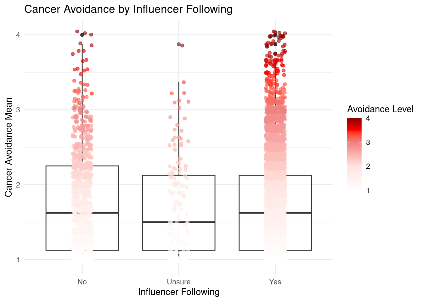
    Influencer_Following = factor(Influencer_Following, levels = c(
    "No",
    "Unsure",
    "Yes")),
    Stressful_Events_Recent = factor(Stressful_Events_Recent, levels = c(
      "No, it was within the last 30 days", 
      "I did not experience a stressful or distressing event within the last 30 days", 
      "Yes, it occurred more than 30 days ago")),
    Current_Depression = factor(Current_Depression, levels = c(
      "Yes",
      "No")),
    Stressful_Events_Detachment = factor(Stressful_Events_Detachment, level = c(
      "Yes",
      "No")),
    Anxiety_Trouble_Relaxing = factor(Anxiety_Trouble_Relaxing, levels = c(
             "Not at all",
             "Several days",
             "More than half the days",
             "Nearly every day")),
    Anxiety_Feeling_Afraid = factor(Anxiety_Feeling_Afraid, levels = c(
             "Not at all",
             "Several days",
             "More than half the days",
             "Nearly every day")),
    Anxiety_Nervousness = factor(Anxiety_Nervousness, levels = c(
             "Not at all",
             "Several days",
             "More than half the days",
             "Nearly every day")),
    Anxiety_Worrying = factor(Anxiety_Worrying, levels = c(
             "Not at all",
             "Several days",
             "More than half the days",
             "Nearly every day")),
    Stressful_Events_Most = factor(Stressful_Events_Most, levels = c(
    "Life-threatening illness or injury",
    "Exposure to toxic substance (for example, dangerous chemicals, radiation)",
    "Sudden accidental death",
    "Transportation accident (for example, car accident, boat accident, train wreck, plane crash)",
    "Serious accident at work, home, or during recreational activity",
    "Captivity (for example, being kidnapped, abducted, held hostage, prisoner of war)",
    "Severe human suffering",
    "Combat or exposure to a war-zone (in the military or as a civilian)",
    "Assault with a weapon (for example, being shot, stabbed, threatened with a knife, gun, bomb)",
    "Sudden violent death (for example, homicide, suicide)",
    "Sexual assault (rape, attempted rape, made to perform any type of sexual act through force or threat of harm)",
    "Serious injury, harm, or death you caused to someone else",
    "Physical assault (for example, being attacked, hit, slapped, kicked, beaten up)",
    "Any other very stressful event or experience",
    "Other unwanted or uncomfortable sexual experience",
    "Fire or explosion",
    "Natural disaster (for example, flood, hurricane, tornado, earthquake)")),
    Fast_Food_Consumption = factor(Fast_Food_Consumption, levels = c(
    "I never eat fast food",
    "Less than once a month",
    "Once a month",
    "2-3 times a month",
    "Once a week or more")),
    Vaccinations = factor(Vaccinations, levels = c(
      "No",
      "It depends",
      "Yes")),
    Meditation = factor(Meditation, levels = c(
    "I've never done this before",
    "I've tried it in the past, but it wasn't for me",
    "I've done this in the past, but not regularly",
    "I did this regularly in the past, but not currently",
    "I do this at least once a month")),
    Physical_Activity_Guidelines = factor(Physical_Activity_Guidelines, levels = c(
        "No, and I do not intend to in the next 6 months.",
        "No, but I intend to in the next 6 months.",
        "No, but I intend to in the next 30 days.",
        "Yes, I have been for LESS than 6 months.",
        "Yes, I have been for MORE than 6 months.")),
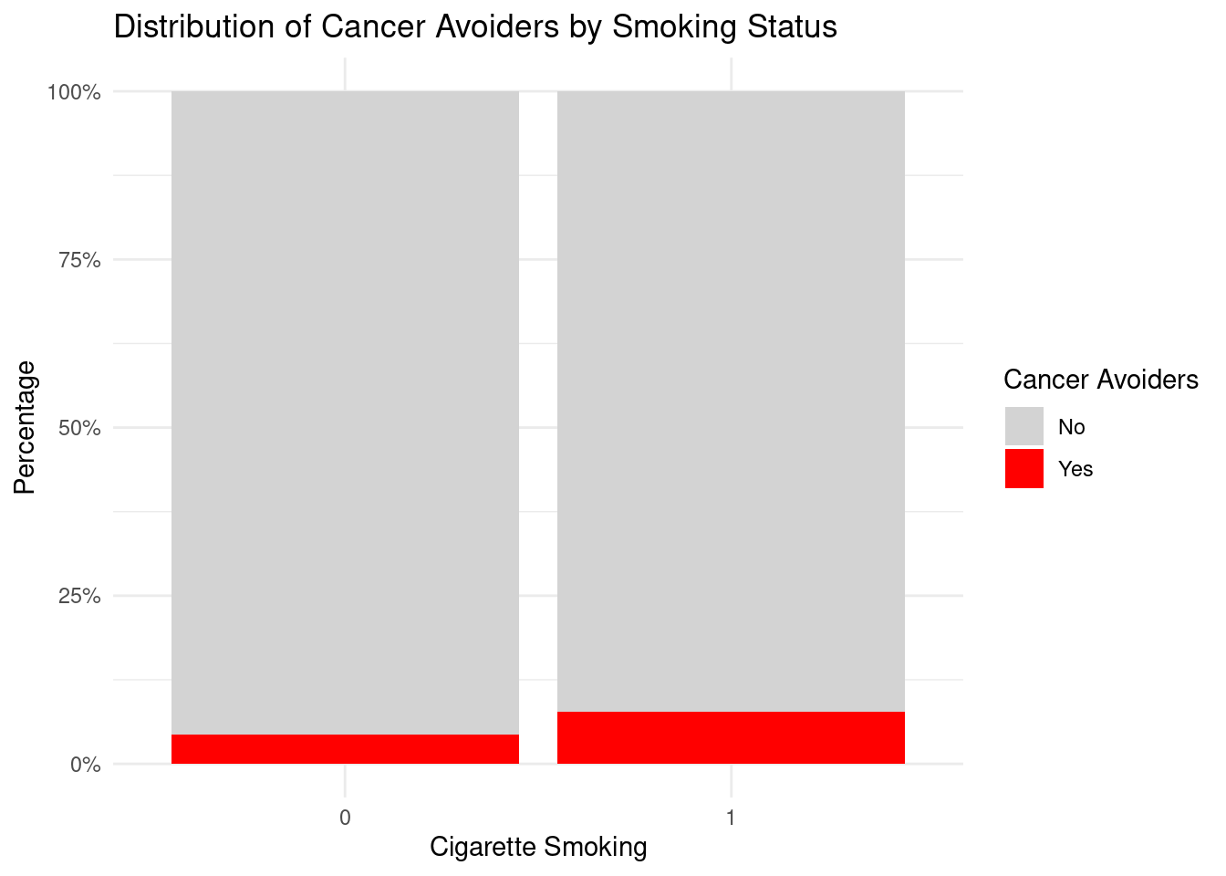
    Cigarette_Smoking = factor(Cigarette_Smoking, levels = c(
        "I don't smoke cigarettes",
        "Less than one a day",
        "1 to 3 cigarettes",
        "4 to 6 cigarettes",
        "7 to 10 cigarettes",
        "More than 10 cigarettes")),
    Supplement_Consumption_Reason = factor(Supplement_Consumption_Reason, levels = c(
        "I do not take any supplements",
        "For maintaining good health in general",
        "For a specific issue")),
    Diet_Type = factor(Diet_Type, levels = c(
        "Vegetarian (I do not eat meat or fish)",
        "Vegan (I do not eat any animal products)",
        "Pollotarian (I do not eat red meat and fish, but eat poultry and fowl)",
        "None of the above",
        "Flexitarian (I eat vegetarian, but also occasionally meat or fish)",
        "Pescetarian (I do not eat meat, but I do eat fish)")),
    Supplement_Consumption = factor(Supplement_Consumption, levels = c(
      "I do not take any supplments", 
      "1", 
      "2", 
      "3", 
      "4 or more")),
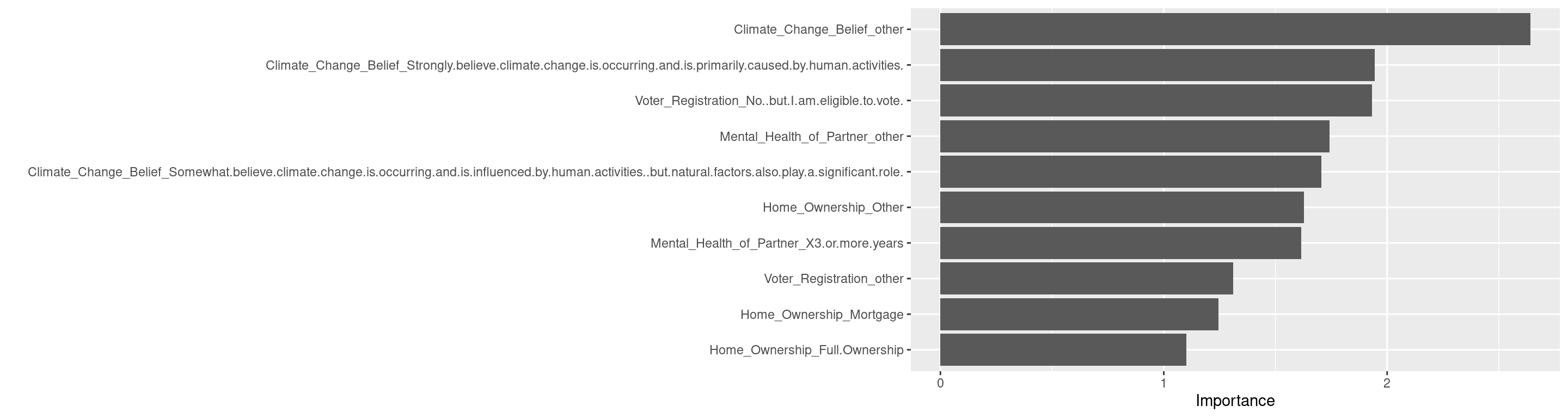
    Home_Ownership = factor(Home_Ownership, levels = c(
    "Rent",
    "Lease",
    "Mortgage",
    "Full Ownership",
    "Other")),
    Voter_Registration = factor(Voter_Registration, levels = c(
        "Yes",
        "No, but I am eligible to vote.",
        "No, and I am not eligible to vote.")),
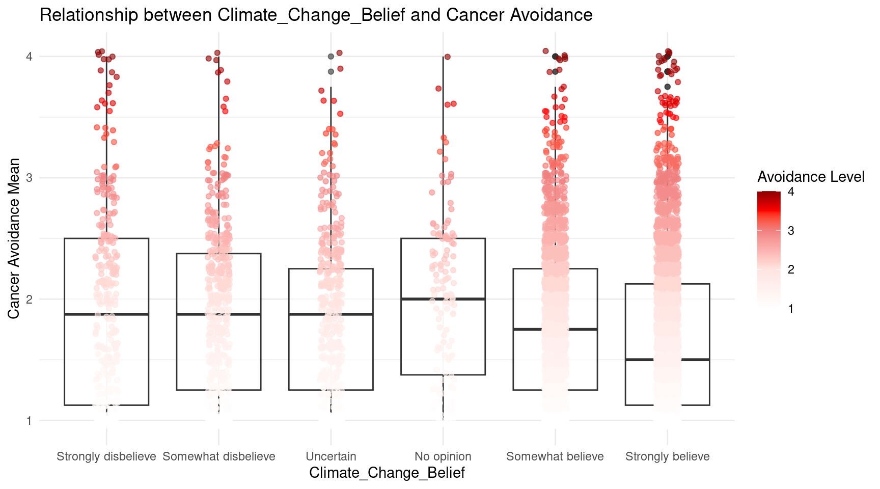
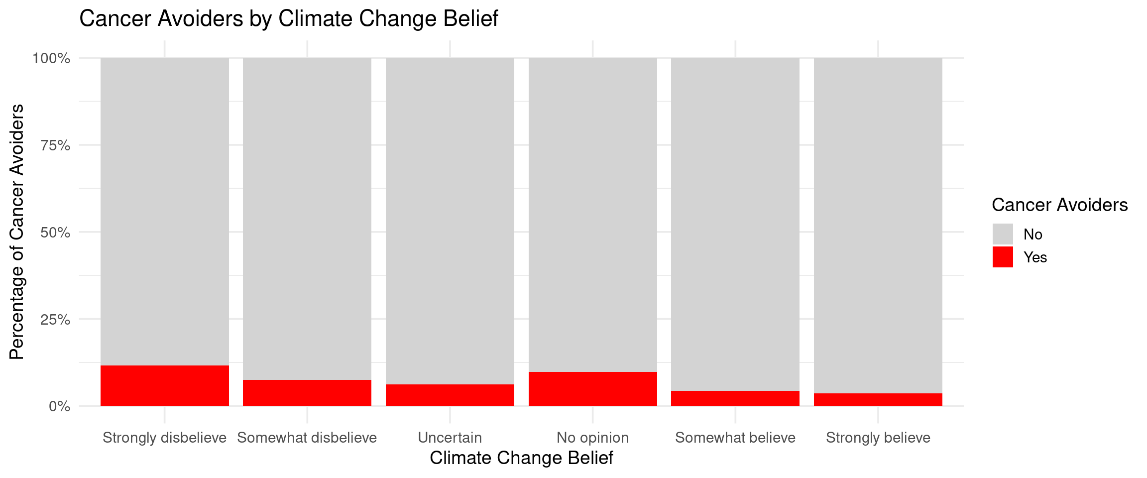
    Climate_Change_Belief = factor(Climate_Change_Belief, levels = c(
        "Strongly skeptical of claims about climate change and its link to human activities.",
        "Somewhat skeptical about the impact of human activities on climate change, believing that climate change is a natural cycle.",
        "Uncertain about the causes and extent of climate change.",
        "No opinion on the matter.",
        "Somewhat believe climate change is occurring and is influenced by human activities, but natural factors also play a significant role.",
        "Strongly believe climate change is occurring and is primarily caused by human activities.")),
    Mental_Health_of_Partner = factor(
      Mental_Health_of_Partner,
      levels = c(
        "My partner has not been diagnosed with a mental illness",
        "Less than a year",
        "1-2 years",
        "2-3 years",
        "3 or more years"
      )
    )
    
)

In [5]:

selectdata <- selectdata %>%
  mutate(
    Job_Classification = recode_factor(Job_Classification,
      `White Collar (e.g., accountant, software developer, human resources manager, marketing analyst, public safety)` = "White Collar",
      `Creative or Cultural (e.g., writer, artist, musician, actor)` = "Creative/Cultural",
      `Public Service and Government (e.g., soldier, teacher, police officer, public health worker, education, childcare)` = "Public Service/Government",
      `Information Technology (e.g., IT specialist, web developer, data scientist, cybersecurity analyst)` = "IT",
      `Service Industry (e.g., retail worker, server, hotel staff, flight attendant, food services, personal care, funeral services, animal/veterinary care, leisure and hospitality)` = "Service Industry",
      `Freelance and Gig Economy (e.g., freelance writer, graphic designer, rideshare driver, delivery person)` = "Freelance/Gig",
      `Blue Collar (e.g., electrician, plumber, mechanic, welder, manufacturing, oil and gas extraction, transportation, utilities, mining, waste collection/treatment/disposal, automotive services)` = "Blue Collar",
      `Professional (e.g., doctor, lawyer, professor, engineer, nurse, healthcare)` = "Professional",
      `I am unemployed/a student/stay at home parent` = "Unemployed/Student/Parent",
      ` Manual Labor (e.g., farmer, construction worker, factory worker, miner, landscaping, agriculture, cleaning and custodial services)` = "Manual Labor"
    )
  )

In [6]:

#  (some of their age greater than 100)

library(ggplot2)

ggplot(selectdata, aes(x = Age)) +
  geom_histogram(binwidth = 5, color = "black") +
  labs(title = "Distribution of Age", x = "Age", y = "Count")

In [7]:

# need renumercing the level

library(ggplot2)

ggplot(selectdata, aes(x = Personal_Income)) +
  geom_bar(fill = "steelblue", color = "black") +
  labs(title = "Distribution of Personal Income", 
       x = "Personal Income", 
       y = "Count") +
  theme_minimal() +
  theme(axis.text.x = element_text(angle = 45, hjust = 1))

In [8]:

selectdata <- selectdata %>%
  mutate(
    Gender4 = case_when(
      Gender == "Woman" ~ "Woman",
      Gender == "Man" ~ "Man",
      Gender == "Non-binary" ~ "Non-binary",
      TRUE ~ "Other"   # all remaining categories go here
    ),
    Gender4 = factor(Gender4, levels = c("Woman", "Man", "Non-binary", "Other")),
    
  Education_Level = case_when(
      Education == "No formal education" ~ 0,
      Education == "Less than a high school diploma" ~ 1,
      Education == "High school graduate - high school diploma or the equivalent (for example: GED)" ~ 2,
      Education == "Some college, but no degree" ~ 3,
      Education == "Associate degree (for example: AA, AS)" ~ 4,
      Education == "Bachelor's degree (for example: BA, AB, BS)" ~ 5,
      Education == "Master's degree (for example: MA, MS, MEng, MEd, MSW, MBA)" ~ 6,
      Education == "Professional degree (for example: MD, DDS, DVM, LLB, JD)" ~ 7,
      Education == "Doctorate degree (for example: PhD, EdD)" ~ 7,      
      Education == "Perfer not to say" ~ 8,
      TRUE ~ NA
    ),
  Age = as.numeric(Age),
  Income = case_when(
    Personal_Income == "Less than $10,000" ~ 1,
    Personal_Income %in% c("$10,000-$19,999", "$20,000-$29,999") ~ 2,
    Personal_Income %in% c("$30,000-$39,999", "$40,000-$49,999") ~ 3,
    Personal_Income %in% c("$50,000-$59,999", "$60,000-$69,999") ~ 4,
    Personal_Income %in% c("$70,000-$79,999", "$80,000-$89,999", "$90,000-$99,999") ~ 5,
    Personal_Income %in% c("$100,000-$124,999", "$125,000-$149,999") ~ 6,
    Personal_Income %in% c("$150,000-$174,999", "$175,000-$199,999", "$200,000-$224,999", 
                           "$225,000-$249,999", "$250,000 or more") ~ 6,
    Personal_Income == "Prefer not to say" ~ 7,
    TRUE ~ NA
  ),
  
    MacArthur_Numeric = as.numeric(gsub("Rung ", "", MacArthur_Scale)),
  
    # Political Party: 1-4
    Political_Party_Group = case_when(
      Political_Party == "Republican" ~ 1,
      Political_Party == "Democrat" ~ 2,
      Political_Party == "Independent" ~ 3,
      Political_Party == "Something else" ~ 4,
      TRUE ~ NA_real_
    ),
    
    # Gender: 1-4
    Gender4 = case_when(
      Gender4 == "Woman" ~ 1,
      Gender4 == "Man" ~ 2,
      Gender4 == "Non-binary" ~ 3,
      Gender4 == "Other" ~ 4,
      TRUE ~ NA_real_
    ),
    
    # Race: white = 1, people of color = 0
    Race2 = case_when(
      Race %in% c("White") ~ 1,
      Race %in% c("American Indian or Alaska Native", "Asian Indian", "Chinese", "Filipino", 
                  "Japanese", "Korean", "Vietnamese", "Samoan", "Guamanian", "Hawaiian", 
                  "Black or African American", "An ethnicity not listed here", "Other") ~ 0,
      TRUE ~ NA_real_
    )
  ) %>%
    filter(Age <= 100)

In [9]:

selectdata <- selectdata %>%
  mutate(
    across(c(Anxiety_Trouble_Relaxing,
             Anxiety_Irritable,
             Anxiety_Restlessness,
             Anxiety_Feeling_Afraid,
             Anxiety_Nervousness,
             Anxiety_Worrying,
             Anxiety_Worrying_Different_Things),
           ~ case_when(
             . == "Not at all" ~ 0,
             . == "Several days" ~ 1,
             . == "More than half the days" ~ 2,
             . == "Nearly every day" ~ 3,
             TRUE ~ NA_real_
           ),
           .names = "{.col}_num"),
    
    # total score (0–21)
    Anxiety_Total_Score = Anxiety_Trouble_Relaxing_num +
                          Anxiety_Irritable_num +
                          Anxiety_Restlessness_num +
                          Anxiety_Feeling_Afraid_num +
                          Anxiety_Nervousness_num +
                          Anxiety_Worrying_num +
                          Anxiety_Worrying_Different_Things_num,
    
    # categorical version
    Anxiety_Severity_cat = case_when(
      Anxiety_Total_Score >= 0  & Anxiety_Total_Score <= 4  ~ "Minimal",
      Anxiety_Total_Score >= 5  & Anxiety_Total_Score <= 9  ~ "Mild",
      Anxiety_Total_Score >= 10 & Anxiety_Total_Score <= 14 ~ "Moderate",
      Anxiety_Total_Score >= 15 & Anxiety_Total_Score <= 21 ~ "Severe",
      TRUE ~ NA_character_
    ),
    
    # numerical version
     Anxiety_Severity_num = case_when(
      Anxiety_Total_Score >= 0  & Anxiety_Total_Score <= 4  ~ 1,
      Anxiety_Total_Score >= 5  & Anxiety_Total_Score <= 9  ~ 2,
      Anxiety_Total_Score >= 10 & Anxiety_Total_Score <= 14 ~ 3,
      Anxiety_Total_Score >= 15 & Anxiety_Total_Score <= 21 ~ 4,
      TRUE ~ NA_real_
    )
  )

In [10]:

selectdata <- selectdata %>%
  mutate(
    across(c(Stressful_Events_Reaction,
             Stressful_Events_Guilt,
             Stressful_Events_Detachment,
             Stressful_Events_Nightmares,
             Stressful_Events_Avoiding_Situations),
           ~ case_when(
             . == "Yes" ~ 1,
             . == "No"  ~ 0,
             TRUE ~ NA_real_
           ),
           .names = "{.col}_num"),
    
    # PC-PTSD-5 score: sum of the 5 recoded items
    PTSD5_Score = Stressful_Events_Reaction_num +
                     Stressful_Events_Guilt_num +
                     Stressful_Events_Detachment_num +
                     Stressful_Events_Nightmares_num +
                     Stressful_Events_Avoiding_Situations_num,
    
    # PTSD5 categorical
    PTSD5_cat = case_when(
      PTSD5_Score == 0 ~ "None",
      PTSD5_Score == 1 ~ "Minimal",
      PTSD5_Score == 2 ~ "Mild",
      PTSD5_Score == 3 ~ "Moderate",
      PTSD5_Score >= 4 ~ "Severe",
      TRUE ~ NA_character_
    )
  )

In [11]:

selectdata <- selectdata %>%
  mutate(
    across(c(Health_Feeling_Failure,
             Health_Hopelessness,
             Health_Feeling_Tired,
             Health_Interest_In_Things,
             Health_Pace,
             Health_Poor_Appetite,
             Health_Thoughts_Of_Self_Infliction,
             Health_Concentration,
             Health_Trouble_Sleeping),
           ~ case_when(
             . == "Not at all" ~ 0,
             . == "Several days" ~ 1,
             . == "More than half the days" ~ 2,
             . == "Nearly every day" ~ 3,
             TRUE ~ NA_real_
           ),
           .names = "{.col}_num"),
    
    # total score (range: 0–27 if 9 items)
    Health_Total_Score = Health_Feeling_Failure_num +
                         Health_Hopelessness_num +
                         Health_Feeling_Tired_num +
                         Health_Interest_In_Things_num +
                         Health_Pace_num +
                         Health_Poor_Appetite_num +
                         Health_Thoughts_Of_Self_Infliction_num +
                         Health_Concentration_num +
                         Health_Trouble_Sleeping_num,
    
    # categorical version
    Health_Depression_Severity = case_when(
      Health_Total_Score >= 0  & Health_Total_Score <= 4   ~ "None to Minimal Depression",
      Health_Total_Score >= 5  & Health_Total_Score <= 9   ~ "Mild Depression",
      Health_Total_Score >= 10 & Health_Total_Score <= 14  ~ "Moderate Depression",
      Health_Total_Score >= 15 & Health_Total_Score <= 19  ~ "Moderately Severe Depression",
      Health_Total_Score >= 20 & Health_Total_Score <= 27  ~ "Severe Depression",
      TRUE ~ NA_character_
    ),
    
    # numeric version of severity
    Health_Depression_Severity_num = case_when(
      Health_Total_Score >= 0  & Health_Total_Score <= 4   ~ 1,
      Health_Total_Score >= 5  & Health_Total_Score <= 9   ~ 2,
      Health_Total_Score >= 10 & Health_Total_Score <= 14  ~ 3,
      Health_Total_Score >= 15 & Health_Total_Score <= 19  ~ 4,
      Health_Total_Score >= 20 & Health_Total_Score <= 27  ~ 5,
      TRUE ~ NA_real_
    )
  )

In [12]:

library(dplyr)
library(stringr)

Attaching package: 'stringr'

The following object is masked from 'package:recipes':

    fixed

library(tidyr)

selectdata <- selectdata %>%
  mutate(
    StressEvents_Count = str_count(Stress_Related_Events, ";") + 1,
    MostStressful_Count = str_count(Stressful_Events_Most, ";") + 1,
    Stress_TotalScore = replace_na(StressEvents_Count, 0) + replace_na(MostStressful_Count, 0)
  )

In [13]:

selectdata <- selectdata %>%
  mutate(
    Cigarette_Smoking_num = case_when(
      Cigarette_Smoking %in% c("Less than one a day", "1 to 3 cigarettes", "4 to 6 cigarettes", "7 to 10 cigarettes", "More than 10 cigarettes") ~ 1,
      Cigarette_Smoking == "I don't smoke cigarettes" ~ 0,
    ),
    Supplement_Consumption_Reason_num = case_when(
      Supplement_Consumption_Reason %in% c("For a specific issue", "For maintaining good health in general") ~ 1,
      Supplement_Consumption_Reason == "I do not take any supplements" ~ 0,
      TRUE ~ NA
    ),
    Meditation_group = factor(
      case_when(
        Meditation == "I've never done this before" ~ "No to past",
        Meditation %in% c("I've tried it in the past, but it wasn't for me",
                          "I've done this in the past, but not regularly",
                          "I did this regularly in the past, but not currently") ~ "Yes to past",
        Meditation == "I do this at least once a month" ~ "Yes to current",
        TRUE ~ NA_character_
    )),
    Facebook_Usage_num = case_when(
      Facebook_Usage == "Daily" ~ 1,
      Facebook_Usage %in% c("Never",
                            "A few times a year",
                            "A few times a month",
                            "At least once a week") ~ 0,
      TRUE ~ NA
    )
)

Health Avoidance

In [14]:

selectdata <- selectdata %>%
  mutate(
    Avoid_Cancer1 = `Information Avoidance - Cancer 1`,
    Avoid_Cancer2 = `Information Avoidance - Cancer 2`,
    Avoid_Cancer3 = `Information Avoidance - Cancer 3 (R)`,
    Avoid_Cancer4 = `Information Avoidance - Cancer 4`,
    Avoid_Cancer5 = `Information Avoidance - Cancer 5 (R)`,
    Avoid_Cancer6 = `Information Avoidance - Cancer 6`,
    Avoid_Cancer7 = `Information Avoidance - Cancer 7 (R)`,
    Avoid_Cancer8 = `Information Avoidance - Cancer 8 (R)`
  )
## the R represent in the Name means reverse code

In [15]:

library(forcats)

# Reorder ALL 8 cancer items at once (1–4, higher = stronger agreement)
selectdata <- selectdata %>%
  mutate(across(starts_with("Avoid_Cancer"),
                ~ as.factor(.) %>%
                  fct_relevel("Strongly disagree",
                              "Somewhat disagree",
                              "Somewhat agree",
                              "Strongly agree") %>%
                  as.numeric()))

The outcome variable, Cancer_Avoidance_Mean, was computed as the average of 8 items measuring participants’ avoidance of cancer-related health information. Four of these items Avoid_Cancer3, Avoid_Cancer5, Avoid_Cancer7, Avoid_Cancer8 were reverse-coded to ensure higher scores consistently reflected greater avoidance. Reverse scoring was calculated using the formula:

Reversed score=(Max+Min)−Original score

In [16]:

selectdata <- selectdata %>%
  mutate(
    Avoid_Cancer3 = 5 - Avoid_Cancer3,
    Avoid_Cancer5 = 5 - Avoid_Cancer5,
    Avoid_Cancer7 = 5 - Avoid_Cancer7,
    Avoid_Cancer8 = 5 - Avoid_Cancer8
  )

Correlation

In [17]:

cancer_items <- select(selectdata, starts_with("Avoid_Cancer"))

# Correlation matrix
cor_matrix <- cor(cancer_items, use = "complete.obs")

print(cor_matrix)

              Avoid_Cancer1 Avoid_Cancer2 Avoid_Cancer3 Avoid_Cancer4
Avoid_Cancer1     1.0000000     0.6631034     0.6184249     0.6069713
Avoid_Cancer2     0.6631034     1.0000000     0.6134200     0.5867422
Avoid_Cancer3     0.6184249     0.6134200     1.0000000     0.5547933
Avoid_Cancer4     0.6069713     0.5867422     0.5547933     1.0000000
Avoid_Cancer5     0.6327710     0.6198924     0.7433590     0.5385642
Avoid_Cancer6     0.6837093     0.5083685     0.4888792     0.5932163
Avoid_Cancer7     0.4873155     0.4906202     0.5815430     0.4147805
Avoid_Cancer8     0.5683388     0.5446571     0.7115237     0.5050828
              Avoid_Cancer5 Avoid_Cancer6 Avoid_Cancer7 Avoid_Cancer8
Avoid_Cancer1     0.6327710     0.6837093     0.4873155     0.5683388
Avoid_Cancer2     0.6198924     0.5083685     0.4906202     0.5446571
Avoid_Cancer3     0.7433590     0.4888792     0.5815430     0.7115237
Avoid_Cancer4     0.5385642     0.5932163     0.4147805     0.5050828
Avoid_Cancer5     1.0000000     0.4906062     0.5565003     0.7388493
Avoid_Cancer6     0.4906062     1.0000000     0.3516696     0.4460674
Avoid_Cancer7     0.5565003     0.3516696     1.0000000     0.5176204
Avoid_Cancer8     0.7388493     0.4460674     0.5176204     1.0000000

In [18]:

library(corrplot)

corrplot 0.95 loaded

corrplot(cor_matrix, 
         method = "color",
         type = "upper",
         order = "original",
         tl.cex = 0.8,
         tl.col = "black",
         tl.srt = 45,
         addCoef.col = "black",
         number.cex = 0.7)

# Alternative visualization with different style
corrplot(cor_matrix, 
         method = "circle",
         type = "full",
         order = "original",
         tl.cex = 0.8,
         tl.col = "black",
         tl.srt = 45,
         col = colorRampPalette(c("blue", "white", "red"))(100))

All the 8 of the cancer items are moderate to high correlate with each other, so we can add them up and get the average score.

Alpha

In [19]:

library(psych)

Attaching package: 'psych'

The following objects are masked from 'package:ggplot2':

    %+%, alpha

The following objects are masked from 'package:scales':

    alpha, rescale

alpha_identity <- psych::alpha(selectdata[, c("Avoid_Cancer1", "Avoid_Cancer2", "Avoid_Cancer3", "Avoid_Cancer4","Avoid_Cancer5", "Avoid_Cancer6", "Avoid_Cancer7", "Avoid_Cancer8")])
print(alpha_identity)

Reliability analysis   
Call: psych::alpha(x = selectdata[, c("Avoid_Cancer1", "Avoid_Cancer2", 
    "Avoid_Cancer3", "Avoid_Cancer4", "Avoid_Cancer5", "Avoid_Cancer6", 
    "Avoid_Cancer7", "Avoid_Cancer8")])

  raw_alpha std.alpha G6(smc) average_r S/N    ase mean   sd median_r
      0.91      0.91    0.91      0.57  10 0.0013  1.7 0.65     0.56

    95% confidence boundaries 
         lower alpha upper
Feldt     0.91  0.91  0.91
Duhachek  0.91  0.91  0.91

 Reliability if an item is dropped:
              raw_alpha std.alpha G6(smc) average_r  S/N alpha se  var.r med.r
Avoid_Cancer1      0.89      0.90    0.89      0.55  8.6   0.0016 0.0098  0.54
Avoid_Cancer2      0.89      0.90    0.90      0.56  9.0   0.0015 0.0107  0.56
Avoid_Cancer3      0.89      0.90    0.89      0.55  8.5   0.0015 0.0085  0.54
Avoid_Cancer4      0.90      0.90    0.90      0.57  9.4   0.0014 0.0104  0.57
Avoid_Cancer5      0.89      0.90    0.89      0.55  8.5   0.0015 0.0079  0.55
Avoid_Cancer6      0.90      0.91    0.90      0.59  9.9   0.0013 0.0070  0.58
Avoid_Cancer7      0.91      0.91    0.91      0.59 10.2   0.0014 0.0070  0.59
Avoid_Cancer8      0.90      0.90    0.90      0.56  9.0   0.0015 0.0083  0.58

 Item statistics 
                  n raw.r std.r r.cor r.drop mean   sd
Avoid_Cancer1 11215  0.85  0.83  0.82   0.78  1.8 0.90
Avoid_Cancer2 11215  0.79  0.80  0.76   0.73  1.6 0.77
Avoid_Cancer3 11215  0.83  0.84  0.83   0.78  1.6 0.74
Avoid_Cancer4 11215  0.78  0.76  0.71   0.69  1.9 0.93
Avoid_Cancer5 11215  0.83  0.84  0.83   0.78  1.6 0.76
Avoid_Cancer6 11215  0.75  0.72  0.68   0.65  2.3 1.02
Avoid_Cancer7 11215  0.67  0.70  0.63   0.59  1.4 0.59
Avoid_Cancer8 11215  0.79  0.80  0.77   0.72  1.7 0.83

Non missing response frequency for each item
              0    1    2    3    4 5 miss
Avoid_Cancer1 0 0.45 0.32 0.18 0.05 0    0
Avoid_Cancer2 0 0.56 0.32 0.10 0.03 0    0
Avoid_Cancer3 0 0.54 0.35 0.09 0.02 0    0
Avoid_Cancer4 0 0.42 0.27 0.26 0.05 0    0
Avoid_Cancer5 0 0.50 0.38 0.10 0.03 0    0
Avoid_Cancer6 0 0.29 0.23 0.36 0.12 0    0
Avoid_Cancer7 0 0.69 0.27 0.03 0.01 0    0
Avoid_Cancer8 0 0.53 0.31 0.12 0.04 0    0

• Based on the analysis, the alpha does not improve for the measure if any of the items are dropped. All final alphas will be equal or lower than the 0.89 raw alpha and 0.9 standardized alpha.

• The internal consistency of the Information Avoidance – Cancer items was high (std.alpha = 0.895), suggesting that the items measured a coherent construct. The average inter-item correlation was (average_r = 0.55), indicating moderately strong associations among the items without redundancy. Reliability estimates (G6 = 0.894) further supported this consistency.

In [20]:

# If one scale:
selectdata <- selectdata %>%
  mutate(Cancer_Avoidance_Mean = rowMeans(cancer_items, na.rm = TRUE))

In [21]:

library(ggplot2)

ggplot(selectdata, aes(x = Cancer_Avoidance_Mean)) +
  geom_histogram(aes(fill = after_stat(x)), binwidth = 0.5, color = "black") +
  scale_x_continuous(
    breaks = seq(1, 4, 0.5),
    limits = c(1, 4)
  ) +
  theme_minimal(base_size = 13) +
  scale_fill_gradientn(
    colours = c("white", "mistyrose", "lightcoral", "red", "darkred"),
    values = scales::rescale(c(1, 2, 3, 3.5, 4)),
    limits = c(1, 4),
    name = "Avoidance Level"
  ) +
  labs(
    x = "Average Cancer Avoidance Score",
    y = "Count",
    title = "Distribution of the Average Cancer Avoidance Score"
  ) +
  theme_minimal(base_size = 13) +
  theme(
    legend.position = "bottom",
    legend.key.width = unit(2, "cm")
  )

Warning: Removed 2 rows containing missing values (`geom_bar()`).

Percentage of participants with Cancer_Avoidance_Mean >= 2.5

In [22]:

# Percentage of participants with Cancer_Avoidance_Mean >= 2.5
mean_25_or_higher <- mean(selectdata$Cancer_Avoidance_Mean >= 2.5, na.rm = TRUE) * 100
mean_25_or_higher

[1] 14.36469

In [23]:

selectdata <- selectdata %>%
  mutate(
    # Binary variable: 1 if mean >= 3 (higher avoidance), 0 if 1–2
    Cancer_Avoiders01 = ifelse(Cancer_Avoidance_Mean >= 3, 1, 0),
    
    # Log transformation (since variable is positive)
    Cancer_Avoidance_log = log10(Cancer_Avoidance_Mean + 1),
    
    # Square root transformation
    Cancer_Avoidance_sqrt = sqrt(Cancer_Avoidance_Mean)
  )

In [24]:

plot_df <- selectdata %>%
  select(Cancer_Avoidance_Mean, Cancer_Avoidance_log, Cancer_Avoidance_sqrt) %>%
  pivot_longer(everything(), names_to = "version", values_to = "value")

# histograms
ggplot(plot_df, aes(x = value)) +
  geom_histogram(bins = 30) +
  facet_wrap(~version, scales = "free") +
  labs(title = "Original vs log vs sqrt", x = NULL, y = "Count")

# densities
ggplot(plot_df, aes(x = value)) +
  geom_density() +
  facet_wrap(~version, scales = "free") +
  labs(title = "Density: original vs log vs sqrt", x = NULL, y = "Density")

In [25]:

write.csv(selectdata, "data/selectdata.csv", row.names = FALSE)

Matrix

In [26]:

library(dplyr)
library(corrplot)
library(knitr)

exclude_patterns <- c("_num$", 
                      paste0("Avoid_Cancer", 1:8),
                      "Cancer_Avoiders01",
                      "Cancer_Avoidance_log",
                      "Cancer_Avoidance_sqrt",
                      "MostStressful_Count")

# Select only numeric vars
numeric_vars_clean <- selectdata %>%
  select(where(is.numeric)) %>%
  select(-matches(paste(exclude_patterns, collapse="|")))

# Recalculate correlation matrix
full_cor_matrix_clean <- cor(numeric_vars_clean, use = "complete.obs")

# Extract correlations with Cancer_Avoidance_Mean
avoidance_corrs <- full_cor_matrix_clean["Cancer_Avoidance_Mean", , drop = FALSE]

# Drop self-correlation
avoidance_corrs <- avoidance_corrs[, colnames(avoidance_corrs) != "Cancer_Avoidance_Mean", drop = FALSE]

# Convert to table
avoidance_corrs_df <- data.frame(
  Variable = colnames(avoidance_corrs),
  Correlation = round(as.numeric(avoidance_corrs), 2)
)

# Print table
knitr::kable(
  avoidance_corrs_df,
  caption = "Correlations of Cancer_Avoidance_Mean with main predictors"
)

Correlations of Cancer_Avoidance_Mean with main predictors

Variable	Correlation
Age	0.03
Gender4	-0.02
Education_Level	-0.06
Income	-0.05
MacArthur_Numeric	-0.08
Political_Party_Group	-0.03
Race2	0.07
Anxiety_Total_Score	0.09
PTSD5_Score	0.09
Health_Total_Score	0.09
StressEvents_Count	0.02
Stress_TotalScore	0.02

In [27]:

library(ggplot2)

ggplot(avoidance_corrs_df, aes(x = reorder(Variable, Correlation), y = Correlation)) +
  geom_col(fill = "steelblue") +
  coord_flip() +
  labs(title = "Correlations of Cancer_Avoidance_Mean with Main Predictors",
       x = "Main Predictors",
       y = "Correlation") +
  theme_minimal(base_size = 12)

REGRESSION MODELS

Random Forest Analysis (tidymodel)

Demographic Model

In [28]:

library(tidymodels)
library(tidyr)
library(vip)

Attaching package: 'vip'

The following object is masked from 'package:utils':

    vi

# need to drop NA to get accuracy
selectdata <- selectdata %>%
  drop_na(
    Cancer_Avoidance_Mean, Ethnicity, Political_Party, Gender4, Job_Classification,
    Education_Level, Age, Income, Race, MacArthur_Numeric
  )


# split into training and testing sets
set.seed(123)
train_idx <- sample(seq_len(nrow(selectdata)), size = 0.7 * nrow(selectdata))
train <- selectdata[train_idx, ]
test  <- selectdata[-train_idx, ]

# Fit random forest model (only for demo)
rf_demo <- rand_forest(
  trees = 500
) %>%
  set_engine("ranger", importance = "impurity") %>% 
  set_mode("regression")

# Set recipe
rf_demo_recipe <- recipe(
  Cancer_Avoidance_Mean ~  Ethnicity + Political_Party + Gender4 + Job_Classification + 
    Education_Level + Age + Income + Race + MacArthur_Numeric, 
  data = train) %>%
  step_other(all_nominal_predictors(), threshold = 0.05) %>%  # collapse rare levels <5%
  step_dummy(all_nominal_predictors()) 

# Create workflow
rf_demo_workflow <- workflow() %>%
  add_model(rf_demo) %>%
  add_recipe(rf_demo_recipe)

# Fit model
rf_demo_fit <- rf_demo_workflow %>%
  fit(data = train)


# Predict on test set
pred <- predict(rf_demo_fit, test) %>%
  bind_cols(test %>% select(Cancer_Avoidance_Mean))


# Model performance
metrics <- pred %>%
  metrics(truth = Cancer_Avoidance_Mean, estimate = .pred)
metrics

# A tibble: 3 × 3
  .metric .estimator .estimate
  <chr>   <chr>          <dbl>
1 rmse    standard      0.635 
2 rsq     standard      0.0163
3 mae     standard      0.529 

# Root Mean Squared Error
rmse <- pred %>%
  rmse(truth = Cancer_Avoidance_Mean, estimate = .pred) %>%
  pull(.estimate)
rmse

[1] 0.6349352

# Mean Absolute Error
mae <- pred %>%
  mae(truth = Cancer_Avoidance_Mean, estimate = .pred) %>%
  pull(.estimate)
mae

[1] 0.5294965

# Correlation between predicted and actual
cor <- cor(pred$.pred, pred$Cancer_Avoidance_Mean)
cor

[1] 0.1278216

# Variable importance
rf_demo_fit %>%
  extract_fit_parsnip() %>%
  vip(num_features = 10)

• RMSE (~0.63) and MAE (~0.53) are pretty close, meaning errors aren’t heavily dominated by outliers.

• Correlation = 0.128 is extremely low. It basically means that predicted values do not track the actual values at all. So the model is not capturing the pattern in the test data.

• If predictors have very weak relationships with the outcome, the model will predicts values near the mean of the training set.

• The random forest model shows that Age is the most predict variable.

In [29]:

age_cancer_linear <- lm(Cancer_Avoidance_Mean ~ Age, data = selectdata)
summary(age_cancer_linear)

Call:
lm(formula = Cancer_Avoidance_Mean ~ Age, data = selectdata)

Residuals:
     Min       1Q   Median       3Q      Max 
-0.79684 -0.59261 -0.08996  0.41156  2.29717 

Coefficients:
             Estimate Std. Error t value Pr(>|t|)    
(Intercept) 1.6740149  0.0227761  73.499  < 2e-16 ***
Age         0.0015164  0.0005817   2.607  0.00915 ** 
---
Signif. codes:  0 '***' 0.001 '**' 0.01 '*' 0.05 '.' 0.1 ' ' 1

Residual standard error: 0.632 on 8092 degrees of freedom
Multiple R-squared:  0.0008391, Adjusted R-squared:  0.0007156 
F-statistic: 6.796 on 1 and 8092 DF,  p-value: 0.009154

• Age coefficient = 0.0015164 meaning for every one year increase in age, the predicted avoidance score goes up by 0.0015164 units.

• Since p-value = 0.009154, so is conventionally significant at the 0.05 level.

• But look at the scatter plot, the trend suggests a slight nonlinear pattern, avoidance rises slowly with age in younger adults, peaks, then decreases slightly in the oldest participants. Despite statistical significance (p = 0.009), the practical effect is very small, as most points cluster near the mean and the trend line is almost flat.

In [30]:

age_cancer_logistic <- glm(Cancer_Avoiders01 ~ Age, data = selectdata, family = binomial)
summary(age_cancer_logistic)

Call:
glm(formula = Cancer_Avoiders01 ~ Age, family = binomial, data = selectdata)

Coefficients:
             Estimate Std. Error z value Pr(>|z|)    
(Intercept) -3.811403   0.180572 -21.107  < 2e-16 ***
Age          0.017472   0.004323   4.042 5.31e-05 ***
---
Signif. codes:  0 '***' 0.001 '**' 0.01 '*' 0.05 '.' 0.1 ' ' 1

(Dispersion parameter for binomial family taken to be 1)

    Null deviance: 2796.0  on 8093  degrees of freedom
Residual deviance: 2780.3  on 8092  degrees of freedom
AIC: 2784.3

Number of Fisher Scoring iterations: 6

• Age coefficient = 0.017472 meaning for every one year increase in age, the predicted avoidance score goes up by 0.017472 units.

• Since p-value = 5.31e-05, so is conventionally significant at the 0.05 level. Which meaning older participants tend to have slightly higher avoidance scores.

• But look at the scatter plot, the trend suggests a slight nonlinear pattern, avoidance rises slowly with age in younger adults, peaks, then decreases slightly in the oldest participants. Despite statistical significance (p = 5.31e-05), the practical effect is very small, as most points cluster near the mean and the trend line is almost flat.

In [31]:

library(ggplot2)

ggplot(data = selectdata, aes(x = Age, y = Cancer_Avoidance_Mean)) +
  geom_point(alpha = 0.6, position = position_jitter(width=20), size = 0.5) +  
  geom_smooth(method = "loess", se = TRUE, color = "red") +  
  labs(x = "Age", 
       y = "Cancer Avoidance Mean",
       title = "Relationship between Age and Cancer Avoidance") +
  scale_x_continuous(limits = c(min(selectdata$Age), 
                              max(selectdata$Age))) +
  theme_minimal()

`geom_smooth()` using formula = 'y ~ x'

Warning: Removed 71 rows containing missing values (`geom_point()`).

Media Use Model

In [32]:

library(tidymodels)
library(tidyr)
library(vip)


# need to drop NA to get accuracy
selectdata <- selectdata %>%
  drop_na(
    Cancer_Avoidance_Mean, Social_Media_Usage, AI_Use, Video_Games_Hours, Listening_Podcasts,
    Facebook_Usage_num, TikTok_Use, X_Twitter_Usage, Social_Media_type, Influencer_Following
  )

# split into training and testing sets
set.seed(123)
train_idx <- sample(seq_len(nrow(selectdata)), size = 0.7 * nrow(selectdata))
train <- selectdata[train_idx, ]
test  <- selectdata[-train_idx, ]

# Fit random forest model (only for demo)
rf_media <- rand_forest(
  trees = 500
) %>%
  set_engine("ranger", importance = "impurity") %>% 
  set_mode("regression")

# Set recipe
rf_media_recipe <- recipe(
  Cancer_Avoidance_Mean ~  Social_Media_Usage + AI_Use + Video_Games_Hours + Listening_Podcasts +
    Facebook_Usage_num + TikTok_Use + X_Twitter_Usage + Influencer_Following,
  data = train) %>%
  step_other(all_nominal_predictors(), threshold = 0.05) %>%  # collapse rare levels <5%
  step_dummy(all_nominal_predictors()) 

# Create workflow
rf_media_workflow <- workflow() %>%
  add_model(rf_media) %>%
  add_recipe(rf_media_recipe)

# Fit model
rf_media_fit <- rf_media_workflow %>%
  fit(data = train)

# Predict on test set
pred <- predict(rf_media_fit, test) %>%
  bind_cols(test %>% select(Cancer_Avoidance_Mean))


# Model performance
metrics <- pred %>%
  metrics(truth = Cancer_Avoidance_Mean, estimate = .pred)
metrics

# A tibble: 3 × 3
  .metric .estimator  .estimate
  <chr>   <chr>           <dbl>
1 rmse    standard   0.620     
2 rsq     standard   0.00000604
3 mae     standard   0.521     

# Root Mean Squared Error
rmse <- pred %>%
  rmse(truth = Cancer_Avoidance_Mean, estimate = .pred) %>%
  pull(.estimate)
rmse

[1] 0.6203144

# Mean Absolute Error
mae <- pred %>%
  mae(truth = Cancer_Avoidance_Mean, estimate = .pred) %>%
  pull(.estimate)
mae

[1] 0.520895

# Correlation between predicted and actual
cor <- cor(pred$.pred, pred$Cancer_Avoidance_Mean)
cor

[1] -0.002456653

# Variable importance
rf_media_fit %>%
  extract_fit_parsnip() %>%
  vip(num_features = 10)

RMSE (~0.6) and MAE (~0.52) are pretty close, meaning errors aren’t heavily dominated by outliers.

Correlation = -0.0024 is extremely low. It basically means that predicted values do not track the actual values at all. So the model is not capturing the pattern in the test data.

If predictors have very weak relationships with the outcome, the model will predicts values near the mean of the training set.

The random forest model shows that Facebook Usage is the most predictive variable.

In [33]:

facebook_cancer_linear <- lm(Cancer_Avoidance_Mean ~ Facebook_Usage_num, data = selectdata)
summary(facebook_cancer_linear)

Call:
lm(formula = Cancer_Avoidance_Mean ~ Facebook_Usage_num, data = selectdata)

Residuals:
     Min       1Q   Median       3Q      Max 
-0.74022 -0.58722 -0.08722  0.41278  2.28778 

Coefficients:
                   Estimate Std. Error t value Pr(>|t|)    
(Intercept)         1.71222    0.01287 133.053   <2e-16 ***
Facebook_Usage_num  0.02800    0.01806   1.551    0.121    
---
Signif. codes:  0 '***' 0.001 '**' 0.01 '*' 0.05 '.' 0.1 ' ' 1

Residual standard error: 0.6294 on 4857 degrees of freedom
Multiple R-squared:  0.0004947, Adjusted R-squared:  0.000289 
F-statistic: 2.404 on 1 and 4857 DF,  p-value: 0.1211

• Facebook Usage coefficient = 0.028 meaning for every one 5 hours increase in facebook usage, the predicted avoidance score goes up by 0.028 units.

• Since p-value = 0.1211, so is not conventionally significant at the 0.05 level.

• But look at the scatter plot,

In [34]:

facebook_cancer_logistic <- glm(Cancer_Avoiders01 ~ Facebook_Usage_num, data = selectdata, family = binomial)
summary(facebook_cancer_logistic)

Call:
glm(formula = Cancer_Avoiders01 ~ Facebook_Usage_num, family = binomial, 
    data = selectdata)

Coefficients:
                   Estimate Std. Error z value Pr(>|z|)    
(Intercept)         -3.3011     0.1104 -29.889   <2e-16 ***
Facebook_Usage_num   0.3189     0.1450   2.199   0.0279 *  
---
Signif. codes:  0 '***' 0.001 '**' 0.01 '*' 0.05 '.' 0.1 ' ' 1

(Dispersion parameter for binomial family taken to be 1)

    Null deviance: 1692.9  on 4858  degrees of freedom
Residual deviance: 1688.0  on 4857  degrees of freedom
AIC: 1692

Number of Fisher Scoring iterations: 6

• For Facebook_Usage_num, there is not a conventionally significant at the 0.05 level.

In [35]:

library(ggplot2)

ggplot(data = selectdata, aes(x = Facebook_Usage_num, y = Cancer_Avoidance_Mean)) +
  geom_point() +
  labs(x = "Facebook Usage", 
       y = "Cancer Avoidance Mean",
       title = "Relationship between Facebook Usage and Cancer Avoidance") +
  theme_minimal()

ggplot(data = selectdata, aes(x = Facebook_Usage_num, y = Cancer_Avoidance_Mean)) +
  geom_point(alpha = 0.6, position = position_jitter(width=0.5), size = 0.5) +  
  geom_smooth(method = "loess", se = TRUE, color = "red") +  
  labs(x = "Facebook Usage", 
       y = "Cancer Avoidance Mean",
       title = "Relationship between Facebook Usage and Cancer Avoidance") +
  scale_x_continuous(limits = c(min(selectdata$Facebook_Usage_num), 
                              max(selectdata$Facebook_Usage_num))) +
  theme_minimal()

`geom_smooth()` using formula = 'y ~ x'

Warning in simpleLoess(y, x, w, span, degree = degree, parametric = parametric,
: pseudoinverse used at -0.005

Warning in simpleLoess(y, x, w, span, degree = degree, parametric = parametric,
: neighborhood radius 1.005

Warning in simpleLoess(y, x, w, span, degree = degree, parametric = parametric,
: reciprocal condition number 8.3096e-31

Warning in simpleLoess(y, x, w, span, degree = degree, parametric = parametric,
: There are other near singularities as well. 1.01

Warning in predLoess(object$y, object$x, newx = if (is.null(newdata)) object$x
else if (is.data.frame(newdata))
as.matrix(model.frame(delete.response(terms(object)), : pseudoinverse used at
-0.005

Warning in predLoess(object$y, object$x, newx = if (is.null(newdata)) object$x
else if (is.data.frame(newdata))
as.matrix(model.frame(delete.response(terms(object)), : neighborhood radius
1.005

Warning in predLoess(object$y, object$x, newx = if (is.null(newdata)) object$x
else if (is.data.frame(newdata))
as.matrix(model.frame(delete.response(terms(object)), : reciprocal condition
number 8.3096e-31

Warning in predLoess(object$y, object$x, newx = if (is.null(newdata)) object$x
else if (is.data.frame(newdata))
as.matrix(model.frame(delete.response(terms(object)), : There are other near
singularities as well. 1.01

Warning: Removed 2414 rows containing missing values (`geom_point()`).

Health Condition Model

In [36]:

library(tidymodels)
library(tidyr)
library(vip)


# need to drop NA to get accuracy
selectdata <- selectdata %>%
  drop_na(
    Cancer_Avoidance_Mean, Stressful_Events_Recent, Current_Depression, Anxiety_Severity_num, PTSD5_Score,
    Health_Depression_Severity_num, Stress_TotalScore
  )


# split into training and testing sets
set.seed(123)
train_idx <- sample(seq_len(nrow(selectdata)), size = 0.7 * nrow(selectdata))
train <- selectdata[train_idx, ]
test  <- selectdata[-train_idx, ]


# Fit random forest model (only for health condition)
rf_health_condition <- rand_forest(
  trees = 500
) %>%
  set_engine("ranger", importance = "impurity") %>% 
  set_mode("regression")


# Set recipe
rf_health_condition_recipe <- recipe(
  Cancer_Avoidance_Mean ~ Stressful_Events_Recent + Current_Depression + Anxiety_Severity_num +
  PTSD5_Score +  Health_Depression_Severity_num + Stress_TotalScore,
  data = train) %>%
  step_other(all_nominal_predictors(), threshold = 0.05) %>%  # collapse rare levels <5%
  step_dummy(all_nominal_predictors()) 


# Create workflow
rf_health_condition_workflow <- workflow() %>%
  add_model(rf_health_condition) %>%
  add_recipe(rf_health_condition_recipe)

# Fit model
rf_health_condition_fit <- rf_health_condition_workflow %>%
  fit(data = train)

# Predict on test set
pred <- predict(rf_health_condition_fit, test) %>%
  bind_cols(test %>% select(Cancer_Avoidance_Mean))


# Model performance
metrics <- pred %>%
  metrics(truth = Cancer_Avoidance_Mean, estimate = .pred)
metrics

# A tibble: 3 × 3
  .metric .estimator .estimate
  <chr>   <chr>          <dbl>
1 rmse    standard     0.631  
2 rsq     standard     0.00294
3 mae     standard     0.534  

# Root Mean Squared Error
rmse <- pred %>%
  rmse(truth = Cancer_Avoidance_Mean, estimate = .pred) %>%
  pull(.estimate)
rmse

[1] 0.6309911

# Mean Absolute Error
mae <- pred %>%
  mae(truth = Cancer_Avoidance_Mean, estimate = .pred) %>%
  pull(.estimate)
mae

[1] 0.5343494

# Correlation between predicted and actual
cor <- cor(pred$.pred, pred$Cancer_Avoidance_Mean)
cor

[1] 0.05421925

# Variable importance
rf_health_condition_fit %>%
  extract_fit_parsnip() %>%
  vip(num_features = 10)

RMSE (~0.63) and MAE (~0.53) are pretty close, meaning errors aren’t heavily dominated by outliers.

Correlation = 0.054 is extremely low. It basically means that predicted values do not track the actual values at all. So the model is not capturing the pattern in the test data.

If predictors have very weak relationships with the outcome, the model will predicts values near the mean of the training set.

The random forest model shows that Stress_TotalScore is the most predict variable.

In [37]:

stress_cancer_linear <- lm(Cancer_Avoidance_Mean ~ Stress_TotalScore, data = selectdata)
summary(stress_cancer_linear)

Call:
lm(formula = Cancer_Avoidance_Mean ~ Stress_TotalScore, data = selectdata)

Residuals:
     Min       1Q   Median       3Q      Max 
-0.74771 -0.61310 -0.09869  0.39410  2.28111 

Coefficients:
                   Estimate Std. Error t value Pr(>|t|)    
(Intercept)        1.750111   0.022151  79.007   <2e-16 ***
Stress_TotalScore -0.002402   0.004419  -0.544    0.587    
---
Signif. codes:  0 '***' 0.001 '**' 0.01 '*' 0.05 '.' 0.1 ' ' 1

Residual standard error: 0.6423 on 2797 degrees of freedom
Multiple R-squared:  0.0001056, Adjusted R-squared:  -0.0002519 
F-statistic: 0.2954 on 1 and 2797 DF,  p-value: 0.5868

In [38]:

stress_cancer_logistic <- glm(Cancer_Avoiders01 ~ Stress_TotalScore, data = selectdata, family = binomial)
summary(stress_cancer_logistic)

Call:
glm(formula = Cancer_Avoiders01 ~ Stress_TotalScore, family = binomial, 
    data = selectdata)

Coefficients:
                   Estimate Std. Error z value Pr(>|z|)    
(Intercept)       -3.011758   0.165814 -18.164   <2e-16 ***
Stress_TotalScore -0.008317   0.033538  -0.248    0.804    
---
Signif. codes:  0 '***' 0.001 '**' 0.01 '*' 0.05 '.' 0.1 ' ' 1

(Dispersion parameter for binomial family taken to be 1)

    Null deviance: 1033.7  on 2798  degrees of freedom
Residual deviance: 1033.7  on 2797  degrees of freedom
AIC: 1037.7

Number of Fisher Scoring iterations: 5

In [39]:

library(ggplot2)

ggplot(data = selectdata, aes(x = Stress_TotalScore, y = Cancer_Avoidance_Mean)) +
  geom_point() +
  labs(x = "Stress_TotalScore", 
       y = "Cancer Avoidance Mean",
       title = "Relationship between Stress_TotalScore and Cancer Avoidance") +
  theme_minimal()

ggplot(data = selectdata, aes(x = Stress_TotalScore, y = Cancer_Avoidance_Mean)) +
  geom_point(alpha = 0.6, position = position_jitter(width=5), size = 0.5) +  
  geom_smooth(method = "loess", se = TRUE, color = "red") +  # Adds a smooth curve
  labs(x = "Stress_TotalScore", 
       y = "Cancer Avoidance Mean",
       title = "Relationship between Stress_TotalScore and Cancer Avoidance") +
  scale_x_continuous(limits = c(min(selectdata$Stress_TotalScore), 
                              max(selectdata$Stress_TotalScore))) +
  theme_minimal()

`geom_smooth()` using formula = 'y ~ x'

Warning: Removed 643 rows containing missing values (`geom_point()`).

Health Behavior Model

In [40]:

library(tidymodels)
library(tidyr)
library(vip)


# need to drop NA to get accuracy
selectdata <- selectdata %>%
  drop_na(
    Cancer_Avoidance_Mean, Fast_Food_Consumption, Meditation_group, Physical_Activity_Guidelines,
    Cigarette_Smoking_num, Supplement_Consumption_Reason_num, Diet_Type, Supplement_Consumption
  )


# split into training and testing sets
set.seed(123)
train_idx <- sample(seq_len(nrow(selectdata)), size = 0.7 * nrow(selectdata))
train <- selectdata[train_idx, ]
test  <- selectdata[-train_idx, ]

# Fit random forest model (only for health_condition)
rf_health_behavior <- rand_forest(
  trees = 500
) %>%
  set_engine("ranger", importance = "impurity") %>% 
  set_mode("regression")


# Set recipe
rf_health_behavior_recipe <- recipe(
  Cancer_Avoidance_Mean ~ Fast_Food_Consumption + Meditation_group + Physical_Activity_Guidelines +
    Cigarette_Smoking_num + Supplement_Consumption_Reason_num + Diet_Type + Supplement_Consumption,
data = train) %>%
  step_other(all_nominal_predictors(), threshold = 0.05) %>%  # collapse rare levels <5%
  step_dummy(all_nominal_predictors()) 


# Create workflow
rf_health_behavior_workflow <- workflow() %>%
  add_model(rf_health_behavior) %>%
  add_recipe(rf_health_behavior_recipe)

# Fit model
rf_health_behavior_fit <- rf_health_behavior_workflow %>%
  fit(data = train)

# Predict on test set
pred <- predict(rf_health_behavior_fit, test) %>%
  bind_cols(test %>% select(Cancer_Avoidance_Mean))


# Model performance
metrics <- pred %>%
  metrics(truth = Cancer_Avoidance_Mean, estimate = .pred)
metrics

# A tibble: 3 × 3
  .metric .estimator .estimate
  <chr>   <chr>          <dbl>
1 rmse    standard     0.644  
2 rsq     standard     0.00616
3 mae     standard     0.534  

# Root Mean Squared Error
rmse <- pred %>%
  rmse(truth = Cancer_Avoidance_Mean, estimate = .pred) %>%
  pull(.estimate)
rmse

[1] 0.6436629

# Mean Absolute Error
mae <- pred %>%
  mae(truth = Cancer_Avoidance_Mean, estimate = .pred) %>%
  pull(.estimate)
mae

[1] 0.5344569

# Correlation between predicted and actual
cor <- cor(pred$.pred, pred$Cancer_Avoidance_Mean)
cor

[1] 0.07847768

# Variable importance
rf_health_behavior_fit %>%
  extract_fit_parsnip() %>%
  vip(num_features = 10)

• RMSE (~0.64) and MAE (~0.53) are pretty close, meaning errors aren’t heavily dominated by outliers.

• Correlation = 0.078 is extremely low. It basically means that predicted values do not track the actual values at all. So the model is not capturing the pattern in the test data.

• If predictors have very weak relationships with the outcome, the model will predicts values near the mean of the training set.

• The random forest model shows that number of Cigarette_Smoking is the most predict variable.

In [41]:

smoking_cancer_linear <- lm(Cancer_Avoidance_Mean ~ Cigarette_Smoking_num, data = selectdata)
summary(smoking_cancer_linear)

Call:
lm(formula = Cancer_Avoidance_Mean ~ Cigarette_Smoking_num, data = selectdata)

Residuals:
     Min       1Q   Median       3Q      Max 
-0.90651 -0.57456 -0.07456  0.42544  2.30044 

Coefficients:
                      Estimate Std. Error t value Pr(>|t|)    
(Intercept)            1.69956    0.01548  109.80  < 2e-16 ***
Cigarette_Smoking_num  0.20695    0.03716    5.57 2.88e-08 ***
---
Signif. codes:  0 '***' 0.001 '**' 0.01 '*' 0.05 '.' 0.1 ' ' 1

Residual standard error: 0.6382 on 2055 degrees of freedom
Multiple R-squared:  0.01487,   Adjusted R-squared:  0.01439 
F-statistic: 31.03 on 1 and 2055 DF,  p-value: 2.882e-08

• Cigarette Smoking coefficient = 0.20695 meaning for every one unit increase in cigarette smoking, the predicted avoidance score goes up by 0.20695 units. So, individuals who smoke more tend to have slightly higher cancer avoidance scores.

• Since p-value = 2.882e-08, so is conventionally significant at the 0.05 level.

In [42]:

smoking_cancer_logistic <- glm(Cancer_Avoiders01 ~ Cigarette_Smoking_num, data = selectdata, family = binomial)
summary(smoking_cancer_logistic)

Call:
glm(formula = Cancer_Avoiders01 ~ Cigarette_Smoking_num, family = binomial, 
    data = selectdata)

Coefficients:
                      Estimate Std. Error z value Pr(>|z|)    
(Intercept)            -3.2575     0.1284 -25.372  < 2e-16 ***
Cigarette_Smoking_num   0.8318     0.2324   3.579 0.000345 ***
---
Signif. codes:  0 '***' 0.001 '**' 0.01 '*' 0.05 '.' 0.1 ' ' 1

(Dispersion parameter for binomial family taken to be 1)

    Null deviance: 751.55  on 2056  degrees of freedom
Residual deviance: 740.02  on 2055  degrees of freedom
AIC: 744.02

Number of Fisher Scoring iterations: 6

• Cigarette Smoking coefficient = 0.8318 meaning for every one unit increase in cigarette smoking, the predicted avoidance score goes up by 0.8318 units. So, individuals who smoke more tend to have slightly higher cancer avoidance scores.

• Since p-value = 0.000345, so is conventionally significant at the 0.05 level.

• Look at the box plot, Smokers show higher cancer avoidance scores on average compared to non-smokers. This could mean that smokers are more aware of or concerned about cancer risks, possibly leading them to engage in other cancer-preventive behaviors or express greater concern about cancer in general.

In [43]:

library(ggplot2)

ggplot(selectdata, aes(x = factor(Cigarette_Smoking_num), y = Cancer_Avoidance_Mean)) +
  geom_boxplot() +
  geom_jitter(width = 0.1, alpha = 0.4, size = 0.7) +
  labs(
    x = "Cigarette Smoking (0 = No, 1 = Yes)",
    y = "Cancer Avoidance Mean",
    title = "Cancer Avoidance by Cigarette Smoking Status"
  ) +
  theme_minimal()

Other Model

In [44]:

library(tidymodels)
library(tidyr)
library(vip)

# need to drop NA to get accuracy
selectdata <- selectdata %>%
  drop_na(
    Cancer_Avoidance_Mean, Home_Ownership, Voter_Registration, Climate_Change_Belief,
    Mental_Health_of_Partner 
  )


# split into training and testing sets
set.seed(123)
train_idx <- sample(seq_len(nrow(selectdata)), size = 0.7 * nrow(selectdata))
train <- selectdata[train_idx, ]
test  <- selectdata[-train_idx, ]

# Fit random forest model (only for other variable)
rf_other <- rand_forest(
  trees = 500
) %>%
  set_engine("ranger", importance = "impurity") %>% 
  set_mode("regression")


# Set recipe
rf_other_recipe <- recipe(
  Cancer_Avoidance_Mean ~ Home_Ownership + Voter_Registration + Climate_Change_Belief +
    Mental_Health_of_Partner,
  data = train) %>%
  step_other(all_nominal_predictors(), threshold = 0.05) %>%  # collapse rare levels <5%
  step_dummy(all_nominal_predictors()) 


# Create workflow
rf_other_workflow <- workflow() %>%
  add_model(rf_other) %>%
  add_recipe(rf_other_recipe)

# Fit model
rf_other_fit <- rf_other_workflow %>%
  fit(data = train)

# Predict on test set
pred <- predict(rf_other_fit, test) %>%
  bind_cols(test %>% select(Cancer_Avoidance_Mean))


# Model performance
metrics <- pred %>%
  metrics(truth = Cancer_Avoidance_Mean, estimate = .pred)
metrics

# A tibble: 3 × 3
  .metric .estimator .estimate
  <chr>   <chr>          <dbl>
1 rmse    standard      0.627 
2 rsq     standard      0.0116
3 mae     standard      0.527 

# Root Mean Squared Error
rmse <- pred %>%
  rmse(truth = Cancer_Avoidance_Mean, estimate = .pred) %>%
  pull(.estimate)
rmse

[1] 0.6273508

# Mean Absolute Error
mae <- pred %>%
  mae(truth = Cancer_Avoidance_Mean, estimate = .pred) %>%
  pull(.estimate)
mae

[1] 0.5265426

# Correlation between predicted and actual
cor <- cor(pred$.pred, pred$Cancer_Avoidance_Mean)
cor

[1] 0.107495

# Variable importance
rf_other_fit %>%
  extract_fit_parsnip() %>%
  vip(num_features = 10)

RMSE (~0.63) and MAE (~0.53) are pretty close, meaning errors aren’t heavily dominated by outliers.

Correlation = 0.107 is extremely low. It basically means that predicted values do not track the actual values at all. So the model is not capturing the pattern in the test data.

If predictors have very weak relationships with the outcome, the model will predicts values near the mean of the training set.

The random forest model shows that Voter Registration (No, but I’m eligiable to vote) is the most predict variable.

In [45]:

voter_cancer_linear <- lm(Cancer_Avoidance_Mean ~ Voter_Registration, data = selectdata)
summary(voter_cancer_linear)

Call:
lm(formula = Cancer_Avoidance_Mean ~ Voter_Registration, data = selectdata)

Residuals:
     Min       1Q   Median       3Q      Max 
-0.89980 -0.59137 -0.09137  0.40863  2.28363 

Coefficients:
                                                     Estimate Std. Error
(Intercept)                                           1.71637    0.01618
Voter_RegistrationNo, but I am eligible to vote.      0.18343    0.05875
Voter_RegistrationNo, and I am not eligible to vote. -0.07351    0.12089
                                                     t value Pr(>|t|)    
(Intercept)                                          106.080  < 2e-16 ***
Voter_RegistrationNo, but I am eligible to vote.       3.122  0.00182 ** 
Voter_RegistrationNo, and I am not eligible to vote.  -0.608  0.54320    
---
Signif. codes:  0 '***' 0.001 '**' 0.01 '*' 0.05 '.' 0.1 ' ' 1

Residual standard error: 0.6339 on 1686 degrees of freedom
Multiple R-squared:  0.006057,  Adjusted R-squared:  0.004878 
F-statistic: 5.137 on 2 and 1686 DF,  p-value: 0.005969

• On average, those eligible but not registered have a cancer avoidance mean 0.18343 points higher than registered voters, and this difference is statistically significant (p = 0.0018).

In [46]:

voter_cancer_logistic <- glm(Cancer_Avoiders01 ~ Voter_Registration, data = selectdata, family = binomial)
summary(voter_cancer_logistic)

Call:
glm(formula = Cancer_Avoiders01 ~ Voter_Registration, family = binomial, 
    data = selectdata)

Coefficients:
                                                     Estimate Std. Error
(Intercept)                                           -3.2373     0.1339
Voter_RegistrationNo, but I am eligible to vote.       0.8903     0.3428
Voter_RegistrationNo, and I am not eligible to vote. -14.3287   747.6478
                                                     z value Pr(>|z|)    
(Intercept)                                          -24.184   <2e-16 ***
Voter_RegistrationNo, but I am eligible to vote.       2.597   0.0094 ** 
Voter_RegistrationNo, and I am not eligible to vote.  -0.019   0.9847    
---
Signif. codes:  0 '***' 0.001 '**' 0.01 '*' 0.05 '.' 0.1 ' ' 1

(Dispersion parameter for binomial family taken to be 1)

    Null deviance: 576.44  on 1688  degrees of freedom
Residual deviance: 568.43  on 1686  degrees of freedom
AIC: 574.43

Number of Fisher Scoring iterations: 16

• On average, those eligible but not registered have a cancer avoidance mean 0.8903 points higher than registered voters, and this difference is statistically significant (p = 0.0094).

• Look at the box plot, There appears to be a modest association between voter registration status and cancer avoidance. Eligible non-registrants show the highest cancer avoidance scores, while registered voters and those ineligible to vote show similar, lower levels. Registered voters shows a heavily concentrated distribution in the lower ranges with many overlapping points.

In [47]:

library(ggplot2)

ggplot(data = selectdata, aes(x = Voter_Registration, y = Cancer_Avoidance_Mean)) +
  geom_boxplot() +  
  geom_jitter(width = 0.1, alpha = 0.4, size = 0.7) +
  labs(x = "Voter_Registration", 
       y = "Cancer Avoidance Mean",
       title = "Relationship between Voter_Registration and Cancer Avoidance") +
  theme_minimal()

In [48]:

sapply(selectdata, function(x) if(is.factor(x)) length(levels(x)) else NA)

                               Ethnicity 
                                       6 
                         Political_Party 
                                       5 
                                  Gender 
                                       7 
                      Job_Classification 
                                      10 
                               Education 
                                      10 
                                     Age 
                                      NA 
                         Personal_Income 
                                      18 
                                    Race 
                                      15 
                         MacArthur_Scale 
                                      10 
                      Social_Media_Usage 
                                       5 
                                  AI_Use 
                                       2 
                       Video_Games_Hours 
                                       6 
                      Listening_Podcasts 
                                       6 
                          Facebook_Usage 
                                       5 
                              TikTok_Use 
                                       4 
                         X_Twitter_Usage 
                                       5 
                       Social_Media_type 
                                    9552 
                    Influencer_Following 
                                       3 
               Stressful_Events_Reaction 
                                       6 
                  Stressful_Events_Guilt 
                                       5 
             Stressful_Events_Detachment 
                                       2 
             Stressful_Events_Nightmares 
                                       6 
    Stressful_Events_Avoiding_Situations 
                                       6 
                 Stressful_Events_Recent 
                                       3 
                      Current_Depression 
                                       2 
                Anxiety_Trouble_Relaxing 
                                       4 
                       Anxiety_Irritable 
                                      11 
                    Anxiety_Restlessness 
                                      11 
                  Anxiety_Feeling_Afraid 
                                       4 
                     Anxiety_Nervousness 
                                       4 
                        Anxiety_Worrying 
                                       4 
                  Health_Feeling_Failure 
                                       9 
                     Health_Hopelessness 
                                       8 
                    Health_Feeling_Tired 
                                      10 
               Health_Interest_In_Things 
                                       8 
                             Health_Pace 
                                       7 
                    Health_Poor_Appetite 
                                       8 
      Health_Thoughts_Of_Self_Infliction 
                                       6 
                    Health_Concentration 
                                       9 
                 Health_Trouble_Sleeping 
                                      11 
       Anxiety_Worrying_Different_Things 
                                      12 
                   Stressful_Events_Most 
                                      17 
                   Stress_Related_Events 
                                    4382 
               Medical_Diagnoses_In_Life 
                                    4862 
                   Fast_Food_Consumption 
                                       5 
            Physical_Activity_Guidelines 
                                       5 
                       Cigarette_Smoking 
                                       6 
           Supplement_Consumption_Reason 
                                       3 
                            Vaccinations 
                                       3 
                               Diet_Type 
                                       6 
                  Supplement_Consumption 
                                       5 
                              Meditation 
                                       5 
                          Home_Ownership 
                                       5 
                      Voter_Registration 
                                       3 
                   Climate_Change_Belief 
                                       6 
                Mental_Health_of_Partner 
                                       5 
        Information Avoidance - Cancer 1 
                                       4 
        Information Avoidance - Cancer 2 
                                       5 
    Information Avoidance - Cancer 3 (R) 
                                       4 
        Information Avoidance - Cancer 4 
                                       4 
    Information Avoidance - Cancer 5 (R) 
                                       5 
        Information Avoidance - Cancer 6 
                                       4 
    Information Avoidance - Cancer 7 (R) 
                                       5 
    Information Avoidance - Cancer 8 (R) 
                                       4 
                                AgeGroup 
                                       6 
                                 Gender4 
                                      NA 
                         Education_Level 
                                      NA 
                                  Income 
                                      NA 
                       MacArthur_Numeric 
                                      NA 
                   Political_Party_Group 
                                      NA 
                                   Race2 
                                      NA 
            Anxiety_Trouble_Relaxing_num 
                                      NA 
                   Anxiety_Irritable_num 
                                      NA 
                Anxiety_Restlessness_num 
                                      NA 
              Anxiety_Feeling_Afraid_num 
                                      NA 
                 Anxiety_Nervousness_num 
                                      NA 
                    Anxiety_Worrying_num 
                                      NA 
   Anxiety_Worrying_Different_Things_num 
                                      NA 
                     Anxiety_Total_Score 
                                      NA 
                    Anxiety_Severity_cat 
                                      NA 
                    Anxiety_Severity_num 
                                      NA 
           Stressful_Events_Reaction_num 
                                      NA 
              Stressful_Events_Guilt_num 
                                      NA 
         Stressful_Events_Detachment_num 
                                      NA 
         Stressful_Events_Nightmares_num 
                                      NA 
Stressful_Events_Avoiding_Situations_num 
                                      NA 
                             PTSD5_Score 
                                      NA 
                               PTSD5_cat 
                                      NA 
              Health_Feeling_Failure_num 
                                      NA 
                 Health_Hopelessness_num 
                                      NA 
                Health_Feeling_Tired_num 
                                      NA 
           Health_Interest_In_Things_num 
                                      NA 
                         Health_Pace_num 
                                      NA 
                Health_Poor_Appetite_num 
                                      NA 
  Health_Thoughts_Of_Self_Infliction_num 
                                      NA 
                Health_Concentration_num 
                                      NA 
             Health_Trouble_Sleeping_num 
                                      NA 
                      Health_Total_Score 
                                      NA 
              Health_Depression_Severity 
                                      NA 
          Health_Depression_Severity_num 
                                      NA 
                      StressEvents_Count 
                                      NA 
                     MostStressful_Count 
                                      NA 
                       Stress_TotalScore 
                                      NA 
                   Cigarette_Smoking_num 
                                      NA 
       Supplement_Consumption_Reason_num 
                                      NA 
                        Meditation_group 
                                       3 
                      Facebook_Usage_num 
                                      NA 
                           Avoid_Cancer1 
                                      NA 
                           Avoid_Cancer2 
                                      NA 
                           Avoid_Cancer3 
                                      NA 
                           Avoid_Cancer4 
                                      NA 
                           Avoid_Cancer5 
                                      NA 
                           Avoid_Cancer6 
                                      NA 
                           Avoid_Cancer7 
                                      NA 
                           Avoid_Cancer8 
                                      NA 
                   Cancer_Avoidance_Mean 
                                      NA 
                       Cancer_Avoiders01 
                                      NA 
                    Cancer_Avoidance_log 
                                      NA 
                   Cancer_Avoidance_sqrt 
                                      NA 

## Can not handle categorical predictors with more than 53 categories. ASk Dr.Shane which variables can be remove, Medical_Diagnoses_In_Life need to be delete (that's too much!)

Multivariate Adaptive Regression Splines (MARS)

Demographic

In [49]:

# Modeling packages
library(earth)     # for fitting MARS models

Loading required package: Formula

Loading required package: plotmo

Loading required package: plotrix

Attaching package: 'plotrix'

The following object is masked from 'package:psych':

    rescale

The following object is masked from 'package:scales':

    rescale

library(caret)     # for automating the tuning process

Loading required package: lattice

Attaching package: 'caret'

The following objects are masked from 'package:yardstick':

    precision, recall, sensitivity, specificity

The following object is masked from 'package:purrr':

    lift

# Model interpretability packages
library(vip)       # for variable importance
library(pdp)       # for variable relationships

Attaching package: 'pdp'

The following object is masked from 'package:purrr':

    partial

In [50]:

# need to drop NA to get accuracy
selectdata <- selectdata %>%
  drop_na(
    Cancer_Avoidance_Mean, Ethnicity, Political_Party, Gender4, Job_Classification,
    Education_Level, Age, Income, Race, MacArthur_Numeric
  )

# split into training and testing sets
set.seed(123)
train_idx <- sample(seq_len(nrow(selectdata)), size = 0.7 * nrow(selectdata))
train <- selectdata[train_idx, ]
test  <- selectdata[-train_idx, ]

# Fit MARS model
mars_model <- earth(
  Cancer_Avoidance_Mean ~ Ethnicity + Political_Party + Gender4 + Job_Classification +
    Education_Level + Age + Income + Race + MacArthur_Numeric,
  data = train
)

# Predict on test set
pred <- predict(mars_model, newdata = test)

summary(mars_model)

Call: earth(formula=Cancer_Avoidance_Mean~Ethnicity+Political_Party+Ge...),
            data=train)

                        coefficients
(Intercept)                1.8673186
Political_PartyDemocrat   -0.1221663
h(3-Education_Level)      -0.1097407
h(MacArthur_Numeric-3)    -0.0342859

Selected 4 of 30 terms, and 3 of 37 predictors
Termination condition: RSq changed by less than 0.001 at 30 terms
Importance: Political_PartyDemocrat, MacArthur_Numeric, Education_Level, ...
Number of terms at each degree of interaction: 1 3 (additive model)
GCV 0.4048718    RSS 472.907    GRSq 0.007560485    RSq 0.01761893

# Variable importance
evimp(mars_model)

                        nsubsets   gcv    rss
Political_PartyDemocrat        3 100.0  100.0
MacArthur_Numeric              2  59.0   72.8
Education_Level                1  11.8   44.3

Political_PartyDemocrat is the most influential predictor (baseline = 100).

MacArthur_Numeric is about 59% as important.

Education_Level is weak (~12%).

In [51]:

library(earth)

mars_model <- earth(
  Cancer_Avoidance_Mean ~ Ethnicity + Political_Party + Gender4 + Job_Classification +
    Education_Level + Age + Income + Race + MacArthur_Numeric,
  data = train,
  degree = 2,       # allow up to 2-way interactions
  nfold = 10,       # 10-fold CV
  keepxy = TRUE
)
summary(mars_model) 

Call: earth(formula=Cancer_Avoidance_Mean~Ethnicity+Political_Party+Ge...),
            data=train, keepxy=TRUE, degree=2, nfold=10)

                                                       coefficients
(Intercept)                                              1.56708813
RaceKorean                                               0.45878852
h(3-Gender4)                                             0.21178348
h(3-Education_Level)                                    -0.15858903
EthnicityPrefer not to say * Political_PartyDemocrat     1.77028451
Political_PartyDemocrat * h(2-Education_Level)           0.82896935
Political_PartyDemocrat * h(5-Income)                   -0.05123354
Job_ClassificationBlue Collar * h(3-MacArthur_Numeric)   0.74256504
RaceWhite * h(MacArthur_Numeric-3)                       0.03677892
h(2-Gender4) * h(Education_Level-3)                     -0.08504094
h(3-Gender4) * h(MacArthur_Numeric-2)                   -0.03174100
h(Education_Level-3) * h(3-Income)                       0.08496109
h(31-Age) * h(MacArthur_Numeric-3)                       0.00588172
h(2-Income) * h(MacArthur_Numeric-3)                    -0.07669137

Selected 14 of 54 terms, and 10 of 37 predictors
Termination condition: Reached nk 75
Importance: Political_PartyDemocrat, EthnicityPrefer not to say, Gender4, ...
Number of terms at each degree of interaction: 1 3 10
GCV 0.4029447  RSS 449.6659  GRSq 0.01228417  RSq 0.06589818  CVRSq -0.07557469

Note: the cross-validation sd's below are standard deviations across folds

Cross validation:   nterms 10.70 sd 4.60    nvars 8.30 sd 2.00

     CVRSq    sd     MaxErr   sd
    -0.076 0.053      -2.43 1.88

summary(mars_model) %>% .$coefficients %>% head(10)

                                                     Cancer_Avoidance_Mean
(Intercept)                                                     1.56708813
EthnicityPrefer not to say*Political_PartyDemocrat              1.77028451
h(3-Education_Level)                                           -0.15858903
Job_ClassificationBlue Collar*h(3-MacArthur_Numeric)            0.74256504
h(Education_Level-3)*h(3-Income)                                0.08496109
h(2-Income)*h(MacArthur_Numeric-3)                             -0.07669137
Political_PartyDemocrat*h(2-Education_Level)                    0.82896935
RaceWhite*h(MacArthur_Numeric-3)                                0.03677892
RaceKorean                                                      0.45878852
h(2-Gender4)*h(Education_Level-3)                              -0.08504094

Interactions appear as products:

EthnicityPrefer not to say * Political_PartyDemocrat = an interaction term between ethnicity and political party.

predictive power is weak: training R-square ~ 0.07, CV R-square: -0.076 This suggests demographic variables don’t explain Cancer_Avoidance_Mean very well.

In [52]:

library(ggplot2)

vip <- evimp(mars_model)

# Convert to data.frame for ggplot
vip_df <- data.frame(
  Variable = rownames(vip),
  GCV = vip[, "gcv"]
)

# Wrap labels at ~20 characters
vip_df$Variable_wrapped <- str_wrap(vip_df$Variable, width = 60)

ggplot(vip_df, aes(x = reorder(Variable_wrapped, GCV), y = GCV)) +
  geom_col(fill = "steelblue") +
  coord_flip() +
  labs(title = "MARS Variable Importance (GCV)",
       x = "Predictor",
       y = "Importance (scaled GCV)")

Visualizing MARS models

In [53]:

plot(mars_model, which = 1)   # Predicted vs observed

The model selection plot shows that both RSq (training fit) and GRSq (generalized R-square) values remain low. This indicates that demographic characteristics provide limited explanatory power for cancer avoidance mean, and adding nonlinear terms does not meaningfully improve predictive accuracy.

Demographics status explain very little of the variation in cancer avoidance. Where effects appear, they are narrow interactions, such as between political affiliation and ethnicity, or between Job_ClassificationBlue Collar and MacArthur_Numeric > 3.

Health condition

In [54]:

# need to drop NA to get accuracy
selectdata <- selectdata %>%
  drop_na(
    Cancer_Avoidance_Mean, Stressful_Events_Recent, Current_Depression, Anxiety_Severity_num, PTSD5_Score,
    Health_Depression_Severity_num, Stress_TotalScore
  )

# split into training and testing sets
set.seed(123)
train_idx <- sample(seq_len(nrow(selectdata)), size = 0.7 * nrow(selectdata))
train <- selectdata[train_idx, ]
test  <- selectdata[-train_idx, ]

# Fit MARS model
mars_model_health_condition <- earth(
    Cancer_Avoidance_Mean ~ Stressful_Events_Recent + Current_Depression + Anxiety_Severity_num +
    PTSD5_Score +  Health_Depression_Severity_num + Stress_TotalScore,
  data = train
)

# Predict on test set
pred <- predict(mars_model_health_condition, newdata = test)

summary(mars_model_health_condition)

Call: earth(formula=Cancer_Avoidance_Mean~Stressful_Events_Recent+Curr...),
            data=train)

                          coefficients
(Intercept)                 1.72758408
h(2-Anxiety_Severity_num)  -0.08617614
h(PTSD5_Score-2)            0.06618512
h(Stress_TotalScore-4)     -0.02304967

Selected 4 of 10 terms, and 3 of 7 predictors
Termination condition: RSq changed by less than 0.001 at 10 terms
Importance: PTSD5_Score, Stress_TotalScore, Anxiety_Severity_num, ...
Number of terms at each degree of interaction: 1 3 (additive model)
GCV 0.4015538    RSS 469.0314    GRSq 0.0156937    RSq 0.02566971

# Variable importance
evimp(mars_model_health_condition)

                     nsubsets   gcv    rss
PTSD5_Score                 3 100.0  100.0
Stress_TotalScore           2  34.1   57.4
Anxiety_Severity_num        1  12.1   37.2

PTSD5_Score is the most influential predictor (baseline = 100).

Stress_TotalScore is about 34% as important.

Anxiety_Severity_num is weak (~12%).

In [55]:

library(earth)

mars_model_health_condition <- earth(
    Cancer_Avoidance_Mean ~ Stressful_Events_Recent + Current_Depression + Anxiety_Severity_num +
    PTSD5_Score +  Health_Depression_Severity_num + Stress_TotalScore,
  data = train,
  degree = 2,       # allow up to 2-way interactions
  nk = 100,
  nfold = 10,       # 10-fold CV
  keepxy = TRUE
)
summary(mars_model_health_condition)

Call: earth(formula=Cancer_Avoidance_Mean~Stressful_Events_Recent+Curr...),
            data=train, keepxy=TRUE, degree=2, nfold=10, nk=100)

                                                                                                                                           coefficients
(Intercept)                                                                                                                                  1.65326477
h(PTSD5_Score-2)                                                                                                                            -0.50585329
h(Stress_TotalScore-7)                                                                                                                      -0.15509138
Stressful_Events_RecentI did not experience a stressful or distressing event within the last 30 days * h(Health_Depression_Severity_num-3)  -0.23699801
Stressful_Events_RecentI did not experience a stressful or distressing event within the last 30 days * h(Stress_TotalScore-5)                0.07697711
h(2-PTSD5_Score) * h(Health_Depression_Severity_num-3)                                                                                       0.37789085
h(PTSD5_Score-2) * h(9-Stress_TotalScore)                                                                                                    0.08780864
h(PTSD5_Score-2) * h(Stress_TotalScore-2)                                                                                                    0.07404818
h(2-Health_Depression_Severity_num) * h(Stress_TotalScore-7)                                                                                 0.18891320
h(Health_Depression_Severity_num-2) * h(Stress_TotalScore-7)                                                                                 0.08373570
h(Health_Depression_Severity_num-3) * h(Stress_TotalScore-3)                                                                                 0.42168698
h(Health_Depression_Severity_num-3) * h(Stress_TotalScore-4)                                                                                -0.55280351

Selected 12 of 51 terms, and 4 of 7 predictors
Termination condition: RSq changed by less than 0.001 at 51 terms
Importance: PTSD5_Score, Stress_TotalScore, Health_Depression_Severity_num, ...
Number of terms at each degree of interaction: 1 2 9
GCV 0.3999687  RSS 450.2396  GRSq 0.0195792  RSq 0.06470649  CVRSq -0.02309585

Note: the cross-validation sd's below are standard deviations across folds

Cross validation:   nterms 3.80 sd 3.43    nvars 2.80 sd 1.14

     CVRSq    sd     MaxErr    sd
    -0.023 0.073       2.34 0.318

pred <- predict(mars_model_health_condition, newdata = test)
rmse <- sqrt(mean((pred - test$Cancer_Avoidance_Mean)^2))
cor(pred, test$Cancer_Avoidance_Mean)

                             [,1]
Cancer_Avoidance_Mean -0.07881039

h(PTSD5_Score-2): When PTSD score > 2, Cancer Avoidance decreases by 0.51.

h(Stress_TotalScore - 7): When stress score > 7, avoidance decreases by 0.16.

Predictive power is weak: training R-square ~ 0.065, The model explains about 6.5% of the variance in Cancer_Avoidance_Mean on the training data and is a weak fit.

CV R-square: -0.023. This suggests health condition variables don’t explain Cancer_Avoidance_Mean ve

The correlation between Cancer_Avoidance_Mean and health condition is also very week (-0.0788)

In [56]:

library(ggplot2)

vip <- evimp(mars_model_health_condition)

# Convert to data.frame for ggplot
vip_df <- data.frame(
  Variable = rownames(vip),
  GCV = vip[, "gcv"]
)

# Wrap labels at ~20 characters
vip_df$Variable_wrapped <- str_wrap(vip_df$Variable, width = 30)

ggplot(vip_df, aes(x = reorder(Variable_wrapped, GCV), y = GCV)) +
  geom_col(fill = "steelblue") +
  coord_flip() +
  labs(title = "MARS Variable Importance (GCV)",
       x = "Predictor",
       y = "Importance (scaled GCV)")

In [57]:

plot(mars_model_health_condition, which = 1)   # Predicted vs observed

The model selection plot shows that both RSq (training fit) and GRSq (generalized R-square) initially increase, indicating that adding the first few hinge functions improves model performance. However, after approximately 4 terms, GRSq reaches its maximum and then slightly declines, suggesting that additional terms provide minimal benefit and may cause overfitting.

The selected model at 4 terms uses 4 predictors and achieves a modest GRSq (0.02), indicating that although weak nonlinear relationships exist, the overall predictive power of the model remains low.

Chae, Jiyoung, Chul-Joo Lee, and Kyungbo Kim. 2019. “Prevalence, Predictors, and Psychosocial Mechanism of Cancer Information Avoidance: Findings from a National Survey of U.S. Adults.” Health Communication 35 (3): 322–30. https://doi.org/10.1080/10410236.2018.1563028.

Dattilo, Taylor M., Caroline M. Roberts, Katherine A. Traino, Dana M. Bakula, Rachel Fisher, Nathan L. Basile, John M. Chaney, and Larry L. Mullins. 2022. “Illness Stigma, Health Anxiety, Illness Intrusiveness, and Depressive Symptoms in Adolescents and Young Adults: A Path Model.” Stigma and Health 7 (3): 311–17. https://doi.org/10.1037/sah0000390.

Emanuel, Amber S., Marc T. Kiviniemi, Jennifer L. Howell, Jennifer L. Hay, Erika A. Waters, Heather Orom, and James A. Shepperd. 2015. “Avoiding Cancer Risk Information.” Social Science & Medicine 147 (December): 113–20. https://doi.org/10.1016/j.socscimed.2015.10.058.

Gigerenzer, Gerd, and Rocio Garcia-Retamero. 2017. “Cassandra’s Regret: The Psychology of Not Wanting to Know.” Psychological Review 124 (2): 179–96. https://doi.org/10.1037/rev0000055.

Ho, Emily H., David Hagmann, and George Loewenstein. 2021. “Measuring Information Preferences.” Management Science 67 (1): 126–45. https://doi.org/10.1287/mnsc.2019.3543.

Howell, Jennifer L., Nikolette P. Lipsey, and James A. Shepperd. 2020. “Health Information Avoidance.” The Wiley Encyclopedia of Health Psychology, September, 279–86. https://doi.org/10.1002/9781119057840.ch77.

Kelly, Christopher. A., and Tali Sharot. 2021. “Individual Differences in Information-Seeking.” Nature Communications 12 (1). https://doi.org/10.1038/s41467-021-27046-5.

O’Brien, Abigail G., William B. Meese, Jennifer M. Taber, Angela E. Johnson, Bianca M. Hinojosa, Raven Burton, Sheemrun Ranjan, Evelyn D. Rodarte, Charlie Coward, and Jennifer L. Howell. 2024. “Why Do People Avoid Health Risk Information? A Qualitative Analysis.” SSM - Qualitative Research in Health 6 (December): 100461. https://doi.org/10.1016/j.ssmqr.2024.100461.

Orom, Heather, Elizabeth Schofield, Marc T Kiviniemi, Erika A Waters, and Jennifer L Hay. 2020. “Agency Beliefs Are Associated with Lower Health Information Avoidance.” Health Education Journal 80 (3): 272–86. https://doi.org/10.1177/0017896920967046.

Song, Shijie, Xinlin Yao, and Nainan Wen. 2021. “What Motivates Chinese Consumers to Avoid Information about the COVID-19 Pandemic?: The Perspective of the Stimulus-Organism-Response Model.” Information Processing & Management 58 (1): 102407. https://doi.org/10.1016/j.ipm.2020.102407.

Soroya, Saira Hanif, and Anthony Faiola. 2023. “Why Did People Avoid Information During the COVID-19 Pandemic? Understanding Information Sources’ Dynamics Among Pakistani Z Generation.” Library Hi Tech 41 (1): 229–47. https://doi.org/10.1108/lht-02-2022-0113.

Sultana, Tahmina, Gurpreet Dhillon, and Tiago Oliveira. 2023. “The Effect of Fear and Situational Motivation on Online Information Avoidance: The Case of COVID-19.” International Journal of Information Management 69 (April): 102596. https://doi.org/10.1016/j.ijinfomgt.2022.102596.

Sweeny, Kate, Darya Melnyk, Wendi Miller, and James A. Shepperd. 2010. “Information Avoidance: Who, What, When, and Why.” Review of General Psychology 14 (4): 340–53. https://doi.org/10.1037/a0021288.

Zhao, Xiaoquan, and Xiaomei Cai. 2009. “The Role of Risk, Efficacy, and Anxiety in Smokers’ Cancer Information Seeking.” Health Communication 24 (3): 259–69. https://doi.org/10.1080/10410230902805932.